

Rigorous Construction of Luttinger Liquids Through Ward Identities |
39 |
5 The First Ward Identity
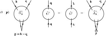
By doing in (3) the chiral gauge transformation (27), one obtains [3] the Ward identity, see Fig. 3,
D+(p)G+2,1(p, k, q) = G+2 (q) − G+2 (k) + +2,1(p, k, q). |
(28) |
2,1
Fig. 3 Graphical representation of the Ward identity (28); the small circle in + represents the function C+ of (30)
We used the definitions |
|
|
|
|
|
|
|
|
|
|
|
|
|
|
|
|
|||||
2,1 |
|
|
|
1 |
|
|
|
|
|
|
|
|
|
|
|
|
|||||
(p, k, q) |
= βL |
|
C |
+ |
(k, k |
− |
|
p) ψ + |
ψ − |
ψ − |
ψ + |
|
T |
(29) |
|||||||
+ |
|
|
|
k |
|
|
|
|
k,+ |
k−p,+; |
|
k,+ |
q,+ |
|
|
|
|||||
|
|
|
|
|
|
|
|
|
|
|
|
|
|
|
|
|
|
|
|
|
|
and |
|
|
|
|
|
|
|
|
|
|
|
|
|
|
|
|
|
|
|
|
|
Cω(k+, k−) = [Ch,0(k−) − 1]Dω (k−) − [Ch,0(k+) − 1]Dω (k+). |
(30) |
||||||||||||||||||||
At graph level, the Ward identities follow from the trivial identity |
|
|
|
||||||||||||||||||
|
|
|
1 |
|
|
1 |
|
|
|
|
|
Dω (p) |
|
|
|
|
|
|
|||
|
|
|
− |
|
|
= |
|
|
. |
|
|
|
(31) |
||||||||
|
Dω (k) |
Dω (k + p) |
Dω (k)Dω (k + p) |
|
|
|
|||||||||||||||
One could guess that the correction term |
|
2,1 |
is negligible. However, this is not |
||||||||||||||||||
|
+ |
||||||||||||||||||||
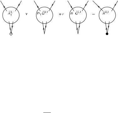
true, but we have the first correction identity where ν+, ν− are O(λ) and weakly dependent on h. Moreover, the term H+2,1 is indeed negligible, in the sense that, if contribution goes to 0 as the external momenta
we can make the limit h → −∞, its |
γ |
h |
). |
|
|
||||
go to 0 (of course staying much larger than |
|
|
|
||||||
If we insert the correction identity in the WI, we get |
|
|
|||||||
(1 |
|
2,1 |
(p, k, q) |
|
|
2,1 |
(p, k, q) |
||
ν+)D+(p)G |
− |
ν−D−(p)G |
|
||||||
|
− |
+ |
|
|
|
− |
(32) |
||
|
= G+2 |
(q) − G+2 (k) + H+2,1(p, k, q). |
|
||||||
40 |
Giuseppe Benfatto |
Fig. 4 The first Correction Identity; the filled point in the last term represents the function |
|
C+(k, k − p) − |
ω νω Dω (p) |
The presence of G2+,1 in the correction identity is not a problem. In fact, this function satisfies another Ward identity and a corresponding correction identity, involving the same constants ν+, ν−, and we get
2,1 |
2,1 |
2,1 |
(p, k, q). |
(33) |
(1 − ν+)D−(p)G− |
(p, k, q) − ν−D+(p)G+ |
(p, k, q) = H− |
2,1
Hence, we can represent G+ as a linear combination of of the formal WI, up to negligible terms.
The first WI can be used to prove that
(2)
Zh1 = 1 + O(εh).
Zh( )
propagators, as in the case
(34)
In order to get this |
result, we put k |
= − |
q |
k, with |
k |
γ h |
. For these values of |
|
2,1 |
|
|
= ¯ |
| ¯ | = |
|
|||
the external momenta, H− |
(p, k, q) is not negligible, but one can show [3] that |
|||||||
|
|
|
|
|
|
|
|
|
|
|
|
2,1 |
(2k¯ |
, k¯ , |
|
k¯ ) |
|
|
|
|
|
|
|
|
|
2h |
|
|||||
|
|
|
|
|
|
|
||||
|
+ |
|
|
|
− |
|
|
≤ Cγ − |
|
εh |
|
|
D+(2k¯ ) |
|
|
|
|
|
|||
Zh(2) |
(35) |
|||
|
|
|
. |
|
(Z |
(1) |
2 |
||
h |
) |
|
|
|
|
|
|
|
|
6 The Second Ward Identity
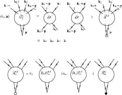
Another WI that plays an important role is that graphically represented in the following picture.
If one inserts this identity in the Dyson equation, the two terms containing the four point function give the right bound, but the correction term 4+,1/D+(p) has the same bad bound as the original one, so making apparently useless the WI. However, there is again a correction identity, see Fig. 6, that allows us to solve this problem.
This identity involves also the correlation function G4−,1; hence, as before, in order to get a relation involving only G4+,1, G4+ and some negligible terms, one has to use also another WI and the corresponding correction identity.
Rigorous Construction of Luttinger Liquids Through Ward Identities |
41 |
Fig. 5 The second Ward Identity; the small circle in the last term represents the function
C+(k, k − p)
Fig. 6 The second Correction Identity; the filled point in the last term represents the function |
|
C+(k, k − p) − |
ω νω Dω (p) |
4,1
However, to show that the contribution of H+ has the right bound is not so simple, since we need to evaluate it for external momenta of order γ h. It turns out that we have to evaluate a correlation very similar to the four point function with one of the external vertices substituted with a suitable “correction vertex”, see [4] for the very technical details.
7 The Euclidean Thirring Model
It is a the Euclidean version of a relativistic two dimensional model, formally defined by the Grassmannian measure
|
− |
|
− ¯ x |
μ |
x + + |
¯ x |
|
x + |
¯ x |
x |
|
|
¯ |
|
|
)2 |
|
||||||||
dψ dψ exp |
|
dx |
ψ |
iγ μ∂ ψ |
|
μψ |
ψ |
|
λ(ψ |
ψ |
(36) |
|
{γ μ, γ ν } = −2δμ,ν . |
|
|
|
|
|
|
|
|
|
(37) |
||
In order to give a meaning to the model, one has to introduce an u.v. and an i.r. cutoff, together with suitable field strength and interaction renormalization.
42 |
Giuseppe Benfatto |
Let us consider the massless case, μ = 0. By a suitable field transformation, one can show that the model can be written as the Tomonaga model with free measure
|
|
|
|
|
|
|
|
|
|
|
|
|
|
|
|
|
|
|
|
|
|
|
|
|
|
|
|
|
|
|
|
|
|
|
|
Z(1) |
|
|
|
|
|
|
|
|
|
|
|
|
|
||||||||||||||
|
|
|
|
|
|
|
|
|
|
|
|
|
|
|
|
|
|
|
|
|
|
|
|
|
|
|
|
|
|
|
|
P (dψ ) |
= |
D ψ exp |
|
|
|
N |
|
|
|
|
|
|
C |
|
(k)( |
ik |
0 + |
ωk)ψ |
|
|
ψ |
|
|
||||||||
|
N |
|
|
− Lβ |
ω |
=± |
1 k |
D |
|
h,N |
|
− |
|
|
|
k,ω |
|
k,ω |
|
||||||||||||
|
|
|
|
|
|
|
|
|
|
|
|
|
|
|
|
|
|
|
|
|
|
|
|
||||||||
|
|
|
|
|
|
|
|
|
|
|
|
|
|
|
|
|
|
|
|
|
|
|
|
|
|
|
|
|
|||
and interaction |
|
|
|
|
|
|
|
|
|
|
|
|
|
|
|
|
|
|
|
|
|
|
|
|
|
|
|
|
|
||
|
|
|
|
V (ψ ) |
= |
λ |
N |
|
|
dx ψ |
+ |
ψ − |
|
ψ + |
ψ − . |
|
|
|
|
|
|
|
|||||||||
|
|
|
|
|
|
|
|
|
|
|
|
|
x,+ |
|
x,+ |
x,− |
x,− |
|
|
|
|
|
|
|
|||||||
The Schwinger functions can be calculated by the generating functional |
|
||||||||||||||||||||||||||||||
|
|
|
|
|
|
|
|
|
|
|
|
|
|
|
|
|
|
|
|
|
|
|
|
|
|
|
|
||||
|
|
|
|
|
|
|
|
|
|
|
|
|
|
|
|
|
|
+ |
ψ − |
φ+ |
ψ − |
|
ψ + φ− |
||||||||
W (φ, J ) = log |
|
P (dψ )e− |
V (ψ ) |
+ |
|
|
|
dx Jx,ω Z(2)ψ |
+ |
||||||||||||||||||||||
|
|
|
|
|
|
ω |
|
|
|
|
N |
x,ω |
|
x,ω + x,ω |
x,ω |
x,ω |
x,ω . |
||||||||||||||
The analysis of the Tomonaga model implies that the cutoffs can be removed if
|
|
|
|
λN = λ ZN(1) |
2 |
|
|
ZN(1) = c1(λ)γ −N η(λ ), |
ZN(2) = c2(λ)γ −N η(λ ), λ = λ−∞(λ) |
||
where ci (λ) are two arbitrary analytic functions such that ci (0) are strictly positive numbers. They have to be chosen by fixing the values of some correlations at finite values of their external momenta. Note that we have essentially already fixed the interaction strength at physical momentum scales of order one; it is given by λ .
In Ref. [5], which we refer to even for relevant references to the huge literature on the Thirring model, it is shown that all the field correlation functions are well defined, in the limit of removed cutoffs, and that they satisfy the Osterwalder–Schrader axioms. Hence, we are able to get results in agreement with known ones, obtained by different techniques. However, our approach can be extended, with a relatively minor effort, to the massive Thirring model (μ > 0), which was up to now an open problem, at least from the point of view of Mathematical Physics.
In order to understand the type of results one can get, let us consider the two point function Sω (k) in the massless case. Simple scaling arguments, based on the structure of its tree expansion after the cutoffs removal, imply that
S |
ω |
(k) |
= |
|
|k|η(λ ) |
f (λ ) |
(38) |
|
|||||||
|
|
|
Dω (k) c1(λ) |
|
|||
where f (λ ) is a suitable analytic function of λ (hence of λ), independent of c1(λ). If we put the renormalization condition
Dω (k)Sω (k) = 1/mη , if |k| = 1 |
(39) |
we get the well known formula