References

Добавил:

Upload Опубликованный материал нарушает ваши авторские права? Сообщите нам.

Вуз:

Национальный исследовательский университет «МИЭТ»

Предмет:

[НЕСОРТИРОВАННОЕ]

Файл:

Diss / 6 - 753p.pdf

Скачиваний:

Добавлен:

27.03.2016

Размер:

15.34 Mб

Скачать

☆

<<< < Предыдущая 23 24 25 26 27 28 29 30 31 32 33 3435 / 6835 36 37 38 39 40 41 42 43 44 45 46 47 > Следующая >>>

284	Paul Fendley and Kareljan Schoutens

cial lattices, but the effect of (approximate) supersymmetry in general is that defects between different domains come at zero (very low) energy cost.

Acknowledgements This work was supported by the foundations FOM and NWO of the Netherlands, by the NSF via the grant DMR-0412956, and by the DOE under grant DEFG02-97ER41027.

j (τ ) = q−1 + 744 + 196884q + 21493760q2 + 864299970q3 + · · ·

(2π iτ ), Im τ >

0, we have modular invariance property, j (τ )

j ( aτ +b ) for

SL(2, Z), and this is the only function, up to the constant term,

satisfying this property and starting with q−1,

1.M. Beccaria and G.F. De Angelis, Phys. Rev. Lett. 94, 100401 (2005). arXiv:cond-mat/ 0407752

2.R. Bott and L.W. Tu, Differential Forms in Algebraic Topology, GTM 82. Springer, New York (1982)

3.P. Fendley and K. Schoutens, Phys. Rev. Lett. 95, 046403 (2005). arXiv:cond-mat/0504595

4.P. Fendley, B. Nienhuis, and K. Schoutens, J. Phys. A 36, 12399 (2003). arXiv:cond-mat/ 0307338

5.P. Fendley, K. Schoutens, and J. de Boer, Phys. Rev. Lett. 90, 120402 (2003). arXiv:hep-th/ 0210161

6.P. Fendley, K. Schoutens, and H. van Eerten, J. Phys. A 38, 315 (2005)

7.L. Huijse, J.H. Halverson, P. Fendley, and K. Schoutens, Phys. Rev. Lett. 101, 146406 (2008)

8.P.W. Kasteleyn, J. Math. Phys. 4, 287 (1963)

9.H. van Eerten, J. Math. Phys. 46, 123302 (2005). arXiv:cond-mat/0509581

10.E. Witten, Nucl. Phys. B 202, 253 (1982)

11.F.Y. Wu, Phys. Rev. 168, 539 (1967)

Convergence of Symmetric Trap Models

in the Hypercube

L.R.G. Fontes and P.H.S. Lima

Abstract We consider symmetric trap models in the d-dimensional hypercube whose ordered mean waiting times, seen as weights of a measure in N , converge to a Þnite measure as d → ∞, and show that the models suitably represented converge to a K process as d → ∞. We then apply this result to get K processes as the scaling limits of the REM-like trap model and the Random Hopping Times dynamics for the Random Energy Model in the hypercube in time scales corresponding to the ergodic regime for these dynamics.

1 Introduction

Trap models have been proposed as qualitative models exhibiting localization and aging (see [13, 7] for early references). In the mathematics literature there has recently been an interest in establishing such results for a varied class of such models (see [11, 4, 5] and references therein). In particular, it has been recognized that scaling limits play an important role in such derivations (see [11, 2, 10, 6] and references therein). It may be argued that such phenomena correspond to related phenomena exhibited by limiting models.

In this paper we consider symmetric trap models in the hypercube whose mean waiting times converge as a measure to a Þnite measure as the dimension diverges,

L.R.G. Fontes

Instituto de Matem‡tica e Estat’stica, Universidade de S‹o Paulo, Rua do Mat‹o 1010, Cidade Universit‡ria, 05508-090 S‹o Paulo SP, Brasil, e-mail: lrenato@ime.usp.br

P.H.S. Lima

Instituto de Matem‡tica e Estat’stica, Universidade de S‹o Paulo, Rua do Mat‹o 1010, Cidade Universit‡ria, 05508-090 S‹o Paulo SP, Brasil, e-mail: plima@ime.usp.br

Partially supported by CNPq grants 475833/2003-1, 307978/2004-4 and 484351/2006-0, and FAPESP grant 2004/07276-2.

Supported by FAPESP grant 2004/13009-7.

V. Sidoraviciusÿ (ed.), New Trends in Mathematical Physics,	285
© Springer Science + Business Media B.V. 2009

286	L.R.G. Fontes and P.H.S. Lima

and show that these models converge weakly. We then apply this result to establish the scaling limits of two dynamics in the hypercube, namely the REM-like trap model and the Random Hopping Times dynamics for the Random Energy Model, in time scales corresponding to the ergodic regime for these dynamics.

1.1 The Model

Let H denote the d-dimensional hypercube, namely H is the graph (V , E ) with

	V = {0, 1}d ,
	E = {(v, v ) V × V : \|x − x \| = 1)},
where \|v − v \| =	d
where \|v − v \| =	i=1 \|v(i) − v (i)\| is the Hamming distance in V .

We will consider symmetric trap models in H , namely continuous time, space inhomogeneous, simple random walks in H , whose transition probabilities (from


each site of H to any of its d nearest neighbors) are uniform. Let γ d						= {γvd , v
V } denote the set of mean waiting times		characterizing the model.
V } denote the set of mean waiting times			d	} by enumerating	V din decreasing
We willd map V onto the set D := {1, . . . , 2				} by enumerating	V din decreasing
order of γ	(with an arbitrary tie breaking rule), and then consider X , the mapped
process. Let
	γ˜ d = {γ˜xd , x D }					(1)

denote the enumeration in decreasing order of γ d , and view it as a Þnite measure in N = {1, 2, . . .}, the positive natural numbers.

We next consider a class of processes which turns out to contain limits of trap models in H as d → ∞, as we will see below. Let N = {(Nt(x))t ≥0, x N } be

i.i.d. Poisson processes of rate 1, with σj(x) the j -th event time of N (x), x N , j ≥ 1, and let T = {T0; Ti(x), i ≥ 1, x N } be i.i.d. exponential random variables of rate 1. N and T are assumed independent. Consider now a Þnite measure γ

supported on N , and for y		¯	=	N	{∞}	let
supported on N , and for y		N		N		let
Γ (t ) = Γ y (t ) = γy T0 +						∞	Nt(x)
Γ (t ) = Γ y (t ) = γy T0 +						γx		Ti(x),	(2)
						x=1	i=1
where, by convention,	0	(x)		= 0 for every x, and γ∞ = 0. We deÞne the
where, by convention,	i=1	Ti		= 0 for every x, and γ∞ = 0. We deÞne the
¯		¯					≥	0
process Y on N starting at y		N as follows. For t						0
y,	if 0 ≤ t < γ (y)T0,
Yt = x,	if Γ (σj(x)−) ≤ t < Γ (σj(x)) for some 1 ≤ j < ∞,								(3)
∞,	otherwise.

Convergence of Symmetric Trap Models in the Hypercube

287

This process, which we here call the K process with parameter γ , was introduced and studied in [10], where it was shown to arise as limits of trap models in the complete graph with n vertices as n → ∞ (see Lemma 3.11 in [10]). In the next section, we derive a similar result for the hypercube. See Theorem 1. This is our main technical result. Then, in the following section, we apply that result to get the scaling limits of the REM-like trap model and the Random Hopping Times dynamics for the REM in ergodic time scales as K processes. See Sect. 3.

2 Convergence to the K Process

Theorem 1. Suppose that, as d → ∞, γ˜ d converges weakly to a ﬁnite measure γ˜

supported on N	0	¯
	, and that Xd converges weakly to a probability measure μ on N .

Then, Xd converges weakly in Skorohod space as d → ∞ to a K process with parameter γ˜ and initial measure μ.

This result extends the analysis performed in [10] for the trap model in the complete graph, with a similar approach (see Lemma 3.11 in [10] and its proof). The extra difÞculty here comes from the fact that the transition probabilities in the hypercube are not uniform in the state space, as is the case in the complete graph. However, all that is indeed needed is an approximate uniform entrance law in Þnite sets of states. This result, a key tool used several times below, is available from [3]. We state it next, in a form suitable to our purposes, but Þrst some notation. Let X denote the embedded chain of Xd and for a given Þxed Þnite subset J of N , let TJ denote the entrance time of X in J , namely,

		TJ = inf{n ≥ 0 : Xn J }.							(4)
Proposition 2 (Corollary 1.5 [3]).
lim		max		P(	= y\|X0 = x) −	1	=	0.	(5)
			J

d	x /J ,y			XTJ		\|J \|
	→∞					\|J \|

Here | · | denotes cardinality.

Remark 3. Corollary 1.5 of [3] is actually more precise and stronger than the above statement, with error of approximation estimates, and holding for J depending on d in a certain manner as well.

Remark 4. Equation (5) is the only fact about the hypercube used in the proof of Theorem 1. This result would thus hold as well for other graphs with the same property. The hypercube has nevertheless been singled out in analyses of dynamics of mean Þeld spin glasses (see above mentioned references), and that is a reason for us to do the same here.

sion that

0 = t0, t1, . . . , tNT

288	L.R.G. Fontes and P.H.S. Lima
2.1 Proof of Theorem 1

The strategy is to approximate Xd for d large by a trap model in the complete

M		= {	1, . . . , M	}	and mean waiting times	{M˜1	˜M }	for
graph with vertex set M						γ	, . . . , γ
M ≤ d large. Let Y	denote the latter process, and let us put Y0						= Y0 1{Y0

M } + W 1{Y0 / M }, with W an independent uniform random variable in M . To accomplish the approximation, we will resort to an intermediate process, which we

Xd , the trap model on

obtained from Xd

next describe. We start by considering ˆ

The

by replacing its set of mean waiting times (seed(1) above) by {γ˜x , x

D }. d,M

intermediate process we will consider is then

restricted to

, denoted X

by observing it only when it is in

this is the Markov process obtained from ˆ

Xd,M when Xd is outside

(with time stopping for ˆ

to Xd,M

The approximations will be strong ones: we will couple X

Xd,M

and ˆ

to Y M , in the spirit of Theorem 5.2 in [10], where the approximation of Y by Y M , needed here as the last step of the argument, was established. In particular, we also couple X0d to Y0 so that the former converges almost surely to the latter as d → ∞.

2.1.1 Coupling of Xd,M and Y M
ˆ
We Þrst look at the embedded chains of Xd,M	and Y M . Let (pd,M )	i,j M	be the
ˆ	ij	i,j M

ˆ = d,M

transition probabilities of the former chain, and let p mini,j M pij . We leave it to the reader to check that there is a coupling between both chains which agrees at each step with probability at least Mpˆ. We resort to such a coupling. Proposition 2

implies that			Mpˆ → 1
			Mpˆ → 1	(6)
for every M Þxed.
as d → ∞ d,M	and Y	M	have the same mean waiting times at each site, we can
X	and Y		have the same mean waiting times at each site, we can
Since ˆ

couple them in such a way that they have the same waiting times at successive visits

		Xd,M and Y M such that
to each site. One may also Þnd a coupling of ˆ			0		0
P(Xd,M	=	Y M )	→	0	(7)
ˆ 0	=	0	→

as d → ∞. Resorting also to that coupling, we get the following result.

Lemma 5. For every T and M ﬁxed, we have

P(Xd,M	=	M	[	] →
ˆ t		Yt , t			1	(8)
				0, T )

as d → ∞.

Proof. Let NT denote the number of jumps of Y M in the time interval [0, T ], and the respective jump times. We conclude from the above discus-

Convergence of Symmetric Trap Models in the Hypercube											289
P(Xd,M	=	Y M , t	[	0, T N	P(Xd,M	=	Y M , i	=	0, 1, . . . , k N	T =	k)
ˆ t	=	t	[	]\| T = k) =	ˆ ti	=	ti	=	\|	T =
				≥	ˆ 0	=	0		ˆ
					P(Xd,M		Y M ) (Mp)k ,				(9)

and the result follows from (6), (7) and dominated convergence (since Mpˆ is bounded above by 1 for all d and M).

dˆ d,M

2.1.2Coupling of X and X

We couple Xd	and	Xd	(the latter process was deÞned at the beginning of the sec-
		ˆ

tion) in the following way. Note that X is their common embedded chain. We then

make the successive sojourn times of X					d	Xd	, starting from the Þrst ones, be
						and ˆ
given by γ˜Xd	0 T0X0 , γ˜Xd		1 T1X1 , . . . and γ˜X0 T0X0 , γ˜X1 T1X1 , . . . , respectively, where
the common	0	1		N , are i.i.d. rate 1 exponential random variables.
	T x	, T x , . . . , x
With a view towards approximating Xd						Xd,M		strongly in Skorohod space,
						and ˆ

we introduce a time distortion function useful for that (see (11) below). For K a

denote the set

{

1, . . . , K

}

, and consider the successive

Þxed positive integer, let K d

d,M

in and out of

K deÞned as follows. Let

entrance and exit times of X and ˆ

τ0 = τ0 = ξ0 = ξ0 = 0 and for i ≥ 1, let

i =

{

≥

: ˆ t

}

= {

≥

i−1 :

ˆ t

}

τi

inf t

Xd,M

inf

τi

Xd,M

/ K

(10)

and similarly deÞne

≥

1 with

Xd replacing

ξi and ξ , i

Xd,M . See Fig. 1 below.

Fig. 1	Trajectories of X	d	and	Xd,M
	Trajectories of X		and	ˆ

Now for T > 0 Þxed, let N = min{i ≥ 1 : τi > T } and deÞne

	ξj +	ξj −ξj
		τj −τj (t − τj ),
λt		ξj +1−ξj
˜	= ξj +		(t − τj ),
		τj +1−τj

ξN + (t − τN ),


if τj		≤	j	for some 0			≤
if τj	< t		τ	for some 0				j < N ,
j	< t	≤	τj	+	1	for some 0		≤	j < N ,	(11)
if τ	< t		τj		1	for some 0			j < N ,

if t ≥ τN .

290	L.R.G. Fontes and P.H.S. Lima

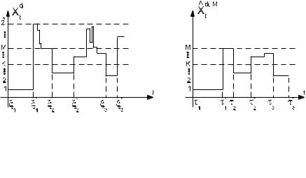
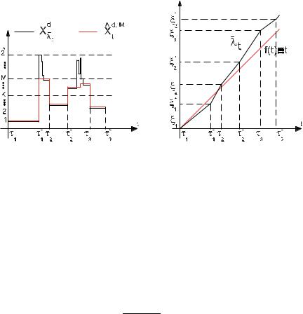
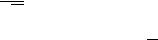
Here and below, we interpret 0/0 as 1. See Fig. 2 below.

Fig. 2	Superimposed trajectories of X	d	λ	Xd,M (left), and superposition
of the	Superimposed trajectories of X		with time distorted by ˜ and	ˆ
of the	λ
	graphs of ˜ and the identity (right)

Remark 6. With the above deÞnition of λ, we Þrst note that Xd,M			Xd whenever
˜	ˆ t	=	λt
any of both processes is visiting K before time τN .		=	˜
any of both processes is visiting K before time τN .

As part of the norm in Skorohod space, we consider the class Λ of nondecreasing Lipschitz functions mapped from [0, ∞) onto [0, ∞), and the following function

on Λ

−

φ (λ)

sup log

λt

λs

(12)

−

We have from (11) above that

0≤s<t

−

ξj

(λ)

max

log

−

max

log

(13)

φ ˜

≤

≤ ≤

−

j −1

−

≤

j N

τj

Below, we will consider the events Aj , j ≥ 0, as follows.

A0 = {X0d K } {there exists 0 ≤ t < ξ1 such that Xtd M \ K },

(14)

Aj = {there exists ξj ≤ t < ξj +1 such that Xtd M \ K }, j ≥ 1.

(15)

It follows from Proposition 2 that for j ≥ 0

lim

inf

(16)

(Aj |Xξj

= x) = 1 − K/M.

→∞

x /M

Notice that the probability on the left hand side of (16) does not depend on j ; we thus get that

Mlim dlim P(Aj ) = 1 uniformly on j ≥ 0.	(17)
→∞ →∞

Convergence of Symmetric Trap Models in the Hypercube

291

2.1.3 Conclusion of proof of Theorem 1
Let DN	( 0,	∞	)) be the (Skorohod) space of c‡dl‡g functions of				[	0,	∞	) to N	with
¯	[	∞					[		∞	¯
metric						∞
			ρ(f, g)	:=	inf φ (λ)	e−uρ(f, g, λ, u)du		,			(18)
				:=	λ Λ	0
where		ρ(f, g, λ, u) := sup [f (t u)]−1 − [g(λ(t ) u)]−1							;
		ρ(f, g, λ, u) := sup [f (t u)]−1 − [g(λ(t ) u)]−1							;		(19)
					t ≥0

see Sect. 3.5 in [9]; Λ and φ were deÞned in the paragraph of (12) above, and

∞−1 = 0.

It follows from Lemma 3.11 in [10] that Y M converges weakly to Y in Skorohod space as M → ∞. In order to prove Theorem 1, it thus sufÞces to show the following result.

Lemma 7. With the above construction of Xd and Y M , we have that for every > 0

Mlim lim sup P(ρ(Xd , Y M ) > ) = 0.	(20)
→∞ d→∞

Proof. Given > 0, let T = − log( /2). Then choosing λ to be the identity, noticing that ρ in (19) is bounded above by 1, and using Lemma 5, we Þnd that for every M > 0

(Xd,M , Y M ) > /2)

≤

P(Xd,M

Y M for some t

[

0, T

)

(21)

(ρ

ˆ t

] →

as d → ∞. So, to establish Lemma 7, it sufÞces to prove Lemma 8 below.

Lemma 8. With above construction of Xd and

Xd,M , we have that for every > 0

lim

(ρ

(Xd,M , Xd ) > )

(22)

lim sup

→∞ d→∞

Proof. Let T = T

= − log , choose K such that |x−1 − y−1| ≤ for every

x, y

K , and consider λ as in (11) with such T and K. Then, by Remark 6

and (12), we see that it sufÞces to show that for every > 0

Mlim

lim sup P

max

log

ξj − ξj

(23)

→∞

j N

τj

→∞

≤ ≤

j −

and

−

ξj

lim

lim sup

max

log

j −1

(24)

−

1 j

≤

τj

→∞ d→∞

≤

j −1

Proof of (23). One readily checks that

292

L.R.G. Fontes and P.H.S. Lima

ξj − ξj

γxd

max

log

max

log

(25)

−

≤

≤ x

1 j

τj

γx

and (23) follows immediately from the assumption that γ˜ d → γ˜ as d → ∞.

Proof of (24). Let γ d,K

γxd,K

γ d

γ d , x

, and consider the trap

d,K

= { ˜

:= ˜d,K ˜K

model X

with mean waiting times γ˜

coupled to X so that both processes

have the same embedded chain X and the respective sojourn times are given by

d,K	X0	d,K	X1	d	X0	d	X1
γ˜X0	T0	, γ˜X1	T1	, . . . and γ˜X0 T0		, γ˜X1 T1		, . . .
		Xd,K denote the process Xd,K restricted to							K	(analogously as Xd,M ),
Let now ˜									K	ˆ	up to
with X its embedded chain. Let N K denote the number of jumps of Xd,K											up to
	˜									˜

time T . Notice that N K is a Poisson process with rate 1/γ˜Kd independent of X and of the history of Xd in the time intervals [ξj , ξj +1), j ≥ 0. Thus, the probability on the left hand side of (24) is bounded above by

> ≤

∞

> P(N K = n),

max K

log

(26)

n 1 j

1≤j ≤N

−

where Uj

j −1

and Vj

−

j −1

. We now estimate the Þrst probability

ξj

τj

on the right hand side of (26). We Þrst note that from (17), and the fact that E(N K )

is Þnite and independent of d, M, we may insert Aj in that probability. We next

write Uj

= Wj + Rj , where Rj is the time spent by Xd in D \ M during the time

interval

, ξj ). From the elementary inequality

log(x

log x

| +

y, valid

[

j −1

+ | ≤ |

for all x, y > 0, we get that

P log

≤ P

+ P Rj > Vj /2

> , Aj

log

> /2, Aj

. (27)

Arguing as in (25) above, we Þnd that the Þrst event in the Þrst probability on the

right hand side of (27) is empty as soon as maxx M \| log	γ˜xd	\| ≤ /2, thus from
right hand side of (27) is empty as soon as maxx M \| log	γx	\| ≤ /2, thus from
	˜

γ˜ d → γ˜ as d → ∞ we only need to consider the second probability on the right hand side of (27). One readily checks that it is bounded above by

max P	Rj > Vj /2	Xd	1	= x	(28)
x /K	Rj > Vj /2	ξj	1	= x	(28)
		−

for all j ≥ 0, and that the above expression does not depend on j . It is enough then to show that for any > 0

P R1 > V1|X0d = x =: Px (R1 > V1) → 0

(29)

as d → ∞ and then M → ∞, uniformly in x > K. This is readily seen to follow from the facts that

max P		(R	1	> )	=	0	(30)
Mlim lim sup x /K	x		1		=
→∞ d→∞

Convergence of Symmetric Trap Models in the Hypercube

293

for any > 0, and that, given δ > 0, there exists > 0 such that
lim sup	max P (V		1 ≤	)	≤	δ.	(31)
M→∞	lim sup x /K	x	1 ≤		≤
M→∞	d→∞

Proof of (30). Let x / K be arbitrary. We will estimate
			d
Ex (R1) := E(R1\|X0d = x) =		y=M+1		γ˜yd Ex (L (y)),			(32)
		y=M+1

where L (y) is the number of visits of X to y from time 0 till its Þrst entrance

in K .

{

}

Let

and consider the discrete time Markov process X such

¯0

y =

{

}

, and let

that X

x and otherwise X is the restriction of X to K

L (y) denote the number of visits of

X to y from time 0 till its Þrst entrance in K .

Clearly,

(y)

(33)

L (y).

}

{

Now let X denote the Markov chain on Ky

with the following set of tran-

sition probabilities. Let p

= (pwz

, w, z Ky {x}), and p

= (pwz, w, z

{

}

, respectively. We

) denote the sets of transition probabilities of X and X

make

max p1

;

x, y

;

y }

(34)

xy =

{

and the remaining pwz2 can be assigned arbitrarily with the only obvious condition that p2 is a set of transition probabilities on Ky . Let L (y) denote the number of visits of X to y from time 0 till its Þrst entrance in K . One readily checks that L (y) is a Geometric random variable with parameter 1 − p and that it stochasti-

cally dominates ¯(y). From this and (33), we conclude that

Ex (L (y)) ≤

(35)

−

uniformly in x / K . Proposition 2 then implies that

lim sup max E (

(y))

≤

(36)

d→∞

x /K x

It follows readily from this, (32) and the assumption that γ˜ d → γ˜ as d → ∞ that

max E		(R	)		1 ∞			γ	,	(37)

				≤ K
lim sup x /K	x	1		≤ K				˜y
d→∞						y=M		+1
						˜	is a Þnite measure on N .
and (30) follows (using MarkovÕs inequality), since γ							is a Þnite measure on N .

294	L.R.G. Fontes and P.H.S. Lima

Proof of (31). Let us Þx x0 / K . Consider the Markov process Z = (Zt )t ≥0 on M such that Z0 = x0, for every x M the waiting time at x before jumping is exponential with mean γ˜x , and the transition probability to y M equals pˆ, if

y /	, and	1−(M−K)pˆ	, if y	K	, where p was deÞned in the paragraph of (6)
K		K		K	ˆ
above.

One readily checks that, given X0d = x0, V1 stochastically dominates S, the time Z spends in M \ K before hitting K for the Þrst time. Since γ˜x is decreasing in x, by the construction of Z, we have that, for every L {K + 1, . . . , M}, S dominates stochastically the random variable γ˜LT 1C , where C is the event that Z visits {K +1, . . . , L} before hitting K for the Þrst time, T is an exponential random variable of rate 1, and 1· is the usual indicator function.

Let now Z denote the embedded chain for Z, and TL = inf{n ≥ 1 : Zn {1, . . . , L}}. Then

P(C|Z0 = x0)

= P(ZTL {K + 1, . . . , L}|ZTL ≤ L, Z0 = x0)

(L − K)pˆ

1 (M K)p

K)p

1 (M L)p

[

−

− ˆ

] +

−

− ˆ

(L − K)Mpˆ

→

(L − K)

−

Mp)M

LMp

as d → ∞ uniformly in x0; see (6).

We conclude that

max P

)

P(γ

)

≤

+ L

lim sup lim sup x /K

˜L

M→∞

d→∞

for every K < L. Thus, given K and δ > 0, we Þrst choose L such that and then > 0 such that P(γ˜LT ≤ ) ≤ δ/2, and we are done.

(38)

(39)

KL ≤ δ/2,

3The REM-Like Trap Model and the Random Hopping Times Dynamics for the REM

In this section we apply Theorem 1 to obtain the scaling limits of two disordered trap models in the hypercube, namely trap models in the hypercube whose mean waiting times are random variables.

3.1 The REM-Like Trap Model

Let τ d := {τvd , v V }, an i.i.d. family of random variables in the domain of attraction of an α-stable law with 0 < α < 1, be the mean waiting times of a trap

Convergence of Symmetric Trap Models in the Hypercube

295

model in H . Let us then consider as before τ˜d := {τ˜xd , x D }, the decreasing order statistics of τ (with an arbitrary tie breaking rule), and let Y d be the mapped process on D .

Now let cd be a scaling factor such that τˆd := cd τ˜d converges to the increments in [0, 1] of an α-stable subordinator. Namely,

inf t

≥

P(τ

> t )

≤

2−d

−1 .

(40)

{

}

Let us now consider Y d

speeded up by

ˆt

Y d (t /c

), t

≥

c−1, namely Y d

Y d

is a trap model on H with mean waiting times given by τ

Notice that ˆ

ˆ = { ˆ

}

denote the increments in

[

0, 1

]

of an α-stable subordinator

Let γ

γi , i

in decreasing order.

ˆ0

Corollary 9. Suppose that Y d converges weakly to a probability measure μ on N .

Then

(41)

(Y d , τ d )

(Y, γ ),

where Y is a K process with parameter γˆ and initial measure μ, and means weak convergence in the product of Skorohod norm and weak convergence norm in the space of ﬁnite measures in N .

Remark 10. In [10], a similar result was proved for the REM-like trap model in the complete graph. See Theorem 5.2 in that reference.

Proof of Corollary 9. We can suppose that we are in a probability space where

d	Theorem 5.2 in [10] for an explicit argument).
τˆ → γˆ almost surely (see proof of
	Y d	Y , and the full result follows.
We can then invoke Theorem 1 to get that ˆ

3.2 Random Hopping Times Dynamics for the REM

This is a dynamics whose equilibrium is the Random Energy Model. Let H d

, v

V }

{Hv

be an i.i.d. family of standard normal random variables, and make

, v

, where τ

β√dHv

and Y

. DeÞning now τ

, τ

, Y

:= {

}

above, with

2 log 2

cd = e−

(42)

+ 2α log d ,

√

with α = 2 log 2/β, we have that, if α < 1, then Corollary 9 holds in this case as well, with γˆ and μ as before.

The proof starts from the known result that in this case τˆd γˆ (see Remark to Theorem 2 in [12]). Again, as in the proof of Corollary 9 above, we can go to a probability space where the latter convergence is almost sure, and close the argument in the same way.

Remark 11. The time scale t time scale mentioned in [8].

→ t /cd adopted in the above models is the ergodic Under shorter scalings (i.e., t → t /cd , with cd cd )

296	L.R.G. Fontes and P.H.S. Lima

the model exhibits aging (when starting from the uniform distribution), and under longer ones (cd cd ), the model reaches equilibrium. More precisely, under shorter scalings, we have that as d → ∞

μ		d		=	Y d ((t	+	d	→	R(s/t ),	(43)
P	d	Y d (t /c	)		Y d ((t		s)/c )		R(s/t ),	(43)

where μd is the initial uniform distribution on D , and R is a nontrivial function such that R(0) = 1 and limx→∞ R(x) = 0. Indeed, for the models of this section (as well as in many other instances in the references), R is the arcsine law:

R(x) =	sin(π α)	1		−α (1 − s)α−1 ds.			(44)
			x s
	π		x s
			1+x		¯		→ ∞
				d	¯	as d	→ ∞	for
See [1]. Under longer scalings, it can be shown that Y d (t /c )					γ	as d		for

every t > 0, where γ¯ is γˆ normalized to be a probability measure. It is the limiting equilibrium measure, or more precisely, the equilibrium measure of Y .

Remark 12. It can be shown that Y exhibits aging at a vanishing time scale (when starting from ∞), i.e.

P∞ (Y ( t ) = Y ( (t + s))) → R(s/t )

(45)

as → 0. See Theorem 5.11 in [10]. This is in agreement with (43).

Acknowledgements This work was mostly done as part of the masterÕs project of the second author, at IME-USP and Þnanced by FAPESP. We thank Claudio Landim for pointing out a mistake in a previous version of this paper.

References

1.	ÿ
1.	G. Ben Arous and V. Cerný, Dynamics of Trap Models. Course at the Les Houches Summer
	School on Mathematical Statistical Physics. Elsevier, Amsterdam (2006)
2.	ÿ	d	. Ann. Probab. 35, 2356Ð2384
2.	G. Ben Arous and J. Cerný, Scaling limit for trap models on Z		. Ann. Probab. 35, 2356Ð2384
	(2007)
3.	G. Ben Arous and V. Gayrard, Elementary potential theory on the hypercube. Electron. J.
	Probab. 13(59), 1726Ð1807 (2008)
4.	G. Ben Arous, A. Bovier, and V. Gayrard, Glauber dynamics of the random energy model. II.
	Aging below the critical temperature. Commun. Math. Phys. 236(1), 1Ð54 (2003)
5.	ÿ
5.	G. Ben Arous, J. Cerný, and T. Mountford Aging, in two-dimensional BouchaudÕs model.
	Probab. Theory Relat. Fields 134, 1Ð43 (2006)
6.	ÿ
6.	G. Ben Arous, A. Bovier, and J. Cerný, Universality of the REM for dynamics of mean-Þeld
	spin glasses. Commun. Math. Phys. 282, 663Ð695 (2008)
7.	J.-P. Bouchaud, Weak ergodicity breaking and aging in disordered systems. J. Phys. I, Fr. 2,
	1705Ð1713 (1992)
8.	J.-P. Bouchaud and D.S. Dean, Aging on ParisiÕs tree. J. Phys. I, Fr. 5, 265Ð286 (1995)
9.	S.N. Ethier and T.G. Kurtz, Markov Processes. Characterization and Convergence. Wiley,
	New York (1986)

Convergence of Symmetric Trap Models in the Hypercube

297

10.L.R.G. Fontes, and P. Mathieu, K-processes, scaling limit and aging for the trap model in the complete graph. Ann. Probab. 36, 1322Ð1358 (2008)

11.L.R.G. Fontes, M. Isopi, and C.M. Newman, Random walks with strongly inhomogeneous rates and singular diffusions: convergence, localization and aging in one dimension. Ann. Probab. 30, 579Ð604 (2002)

12.A. Galves, S. Mart’nez, and P. Picco, Fluctuations in DerridaÕs random energy and generalized random energy models. J. Stat. Phys. 54, 515Ð529 (1989)

13.T.M. Nieuwenhuizen and M.H. Ernst, Excess noise in a hopping model for a resistor with quenched disorder. J. Stat. Phys. 41, 773Ð801 (1985)

Spontaneous Replica Symmetry Breaking in the Mean Field Spin Glass Model

Francesco Guerra

Abstract We give a short review about recent results in the study of the mean ﬁeld Sherrington-Kirkpatrick model for a spin glass. Our methods are essentially based on interpolation and comparison arguments for families of Gaussian random variables. In particular we show how to control the inﬁnite volume limit for the free energy density, and how to relate the model to its replica symmetric approximation. We discuss also the mechanism of replica symmetry breaking, by using suitable interpolation methods. Our results are in agreement with those obtained in the frame of the replica trick through the Parisi Ansatz. Finally, we point out some possible further developments of the theory.

1 Introduction

More than thirty years ago, David Sherrington and Scott Kirkpatrick introduced a celebrated mean ﬁeld model for spin glasses [27, 18], then considered to be a “solvable model”.

It is hard to overestimate the impact of this model on the theoretical physics research. During the three decades after its introduction, hundreds and hundreds of papers have been devoted to the study of its properties, even through numerical methods.

The relevance of the model surely comes from the fact that it is able to represent successfully, at least at the level of the mean ﬁeld approximation, some important features of the physical spin glass systems, of great interest for their peculiar properties.

Let us recall that some dilute magnetic alloys, called spin glasses, are extremely interesting systems from a physical point of view. Their peculiar feature is to exhibit

Francesco Guerra

Department of Physics, Sapienza University of Rome and INFN, Section of Roma 1, Rome, Italy, e-mail: francesco.guerra@roma1.infn.it

V. Sidoraviciusˇ (ed.), New Trends in Mathematical Physics,	299
© Springer Science + Business Media B.V. 2009

300	Francesco Guerra

a new magnetic phase, where magnetic moments are frozen into disordered equilibrium orientations, without any long-range order. We refer for example to [33] and [29] for general reviews about the physical properties of spin glasses. The experimental laboratory investigation about concrete spin glasses is a very difﬁcult subject, because of their peculiar properties. In particular, these materials have some very slowly relaxing modes, with consequent memory effects. Therefore, even the very basic physical concept of a system at thermodynamical equilibrium, at a given temperature, meets a difﬁcult empirical realization.

From a theoretical point of view, some models have been proposed, attempting to capture the essential physical features of spin glasses, in the frame of very simple assumptions.

The basic model has been proposed by Edwards and Anderson [5] many years ago. It is a simple extension of the well-known nearest neighbour Ising model for ferromagnetism to the spin glass case. Consider a large region Λ of the unit lattice in d dimensions. Let us associate an Ising spin σ (n) to each lattice site n. Then, we introduce the lattice Edwards-Anderson Hamiltonian

HΛ(σ, J ) = −	J (n, n )σ (n)σ (n ).
	(n,n )

Here, the sum runs over all couples of nearest neighbour sites in Λ, and J are quenched random couplings, assumed for simplicity to be independent identically distributed random variables, with centered unit Gaussian distribution. The quenched character of the J means that they do not participate in the thermodynamic equilibrium, but act as a kind of random external noise on the coupling of the σ variables. In the expression of the Hamiltonian, we have indicated with σ the set of all σ (n), and with J the set of all J (n, n ). The region Λ must be taken very large, letting it invade the whole lattice in the limit. The physical motivation for this choice is that for real spin glasses, due to quantum interference effects, the effective interaction between the ferromagnetic domains dissolved in the matrix of the alloy oscillates in sign according to distance. This feature is taken into account in the model through the random character of the couplings between spins.

Even though very drastic simpliﬁcations have been introduced in the formulation of this model, as compared to the extremely more complicated nature of physical spin glasses, nevertheless a rigorous study of all properties emerging from the static and dynamic behavior of a thermodynamic system of this kind is far from being complete. In particular, with reference to static equilibrium properties, it is not possible yet to reach a completely substantiated description of the phases emerging in the low temperature region. Even by relying on physical intuition, we get completely different answers from different people working in the ﬁeld.

It is very well known that a mean-ﬁeld version can be associated to the ordinary ferromagnetic Ising model (see for example [28]). The same is possible for the disordered model described by the Edwards-Anderson Hamiltonian deﬁned above. Now we consider a number of sites i = 1, 2, . . . , N , not organized in a lattice, and

Spontaneous Replica Symmetry Breaking

301

let each spin σ (i) at site i interact with all other spins, in the presence of a quenched noise Jij . The precise form of the Hamiltonian will be given in Sect. 2.

This is the mean ﬁeld model for spin glasses, introduced by David Sherrington and Scott Kirkpatrick.

There is also an additional very important reason for the relevance of this model, and related ones. In fact, recently it has become progressively clear that disordered systems of the Sherrington-Kirkpatrick type, and their generalizations, seem to play a very important role for theoretical and practical applications to hard optimization problems, as it is shown for example by Marc Mézard, Giorgio Parisi and Riccardo Zecchina in [22].

It is interesting to remark that the original paper was entitled “Solvable Model of a Spin-Glass”, while a previous draft, according to what recalled by David Sherrington, contained even the stronger denomination “Exactly Solvable”. However, it turned out that the very natural solution devised by the authors is valid only at high temperatures, or for large external magnetic ﬁelds. At low temperatures, the proposed solution exhibits a nonphysical drawback given by a negative entropy, as properly recognized by the authors in their very ﬁrst paper.

It took a few years to ﬁnd an acceptable solution. This was done by Giorgio Parisi in a series of papers, by marking a radical departure from the previous methods. In fact, a very deep method of “spontaneous replica symmetry breaking” was developed. As a consequence the physical content of the theory was encoded in a functional order parameter of new type, and a remarkable structure began to show up for the pure states of the theory, characterized by a kind of hierarchical, ultrametric organization. These very interesting developments, due to Giorgio Parisi, and his coworkers, are explained in a challenging way in the classical book [20]. Part of this structure will be recalled in the following.

It is important to remark that the Parisi solution is presented in the form of an ingenious and clever Ansatz. Until a few years ago it was not known whether this Ansatz would give the true solution for the model, in the so-called thermodynamic limit, when the size of the system becomes inﬁnite, or it would be only a very good approximation to the true solution.

The general structures offered by the Parisi solution, and their possible generalizations for similar models, exhibit an extremely rich and interesting mathematical content. In a very signiﬁcant way, Michel Talagrand inserted a strongly suggestive sentence in the title to his recent book [31]: “Spin glasses: a challenge for mathematicians”.

As a matter of fact, the problem of giving a proper mathematical understanding of the spin glass structure is extremely difﬁcult. In this talk, we would like to recall the main features of a very powerful method, yet extremely simple in its very essence, based on comparison and interpolation arguments on families of Gaussian random variables.

The method found its ﬁrst simple application in [10], where it was shown that the Sherrington-Kirkpatrick replica symmetric approximate solution is a rigorous lower bound for the quenched free energy of the system, uniformly in the size, for any value of the temperature and the external magnetic ﬁeld. Then, it was possible

302	Francesco Guerra

to reach a long awaited result [15]: the convergence of the free energy density in the thermodynamic limit, by an intermediate step where the quenched free energy was shown to be subadditive in the size of the system.

Moreover, still by a generalized interpolation on families of Gaussian random variables, the ﬁrst mentioned result, on the replica symmetric solution, was extended to give a rigorous proof that the expression given by the Parisi Ansatz is also a lower bound for the quenched free energy of the system, uniformly in the size [12]. The method gives not only the bound, but also the explicit form of the correction terms in the form of a sum rule. As a recent and very important result, Michel Talagrand has been able to dominate these correction terms, showing that they vanish in the thermodynamic limit. This extraordinary achievement was ﬁrstly announced in a short note [30], containing only a synthetic sketch of the proof, and then presented with all details in a long paper in Annals of Mathematics [32].

The interpolation method is also at the basis of the far-reaching generalized variational principle proven by Michael Aizenman, Robert Sims and Shannon Starr in [1].

In this lecture, we will concentrate mostly on the main questions connected with the free energy. In particular, we will consider the subadditivity with respect to the system size, the existence of the inﬁnite-volume limit, the broken replica symmetry sum rules and bounds, and the Parisi variational principle. Our treatment will be as simple as possible, by relying on the basic structural properties, and by describing methods of presumably very long lasting power.

The organization of the paper is as follows. In Sect. 2 we explain the basic features of the mean ﬁeld spin glass models, by introducing all necessary deﬁnitions. In next Sect. 3 we give a simple application of the interpolation method to the meanﬁeld spin glass model. In particular, we show the sub-additivity of the quenched free energy with respect to the system size, and the existence of the inﬁnite-volume limit [15].

Section 4 is devoted to a description of the main features of the Parisi representation for the free energy and to its rigorous establishment.

Section 5 will be devoted to some conclusion and outlook for future foreseen developments.

In conclusion, the author would like to thank the organizers of the 2006 Rio de Janeiro International Congress of Mathematical Physics, in particular Vladas Sidoravicius, for the kind invitation and exquisite hospitality to an event full of scientiﬁc, cultural and human content, in a so beautiful surrounding.

2 The Mean Field Spin Glass Model. Basic Deﬁnitions

As in the ferromagnetic mean ﬁeld case, the generic conﬁguration of the mean ﬁeld spin glass model is deﬁned through Ising spin variables σi = ±1, attached to each site i = 1, 2, . . . , N .

Spontaneous Replica Symmetry Breaking

303

But now there is also an external quenched disorder given by the N (N − 1)/2 independent and identical distributed random variables Jij , deﬁned for each couple of sites. For the sake of simplicity, we assume each Jij to be a centered unit Gaussian with averages E(Jij ) = 0, E(Jij2 ) = 1. By quenched disorder we mean that the J have a kind of stochastic external inﬂuence on the system, without participating to the thermal equilibrium.

Now the Hamiltonian of the model is given by the mean ﬁeld expression

1
HN (σ, J ) = − √N (i,j ) Jij σi σj .	(1)

√

Here, the sum runs over all couples of sites. Notice that the term N is necessary in order to ensure a good thermodynamic behavior to the free energy, extensive in the system size. For the sake of simplicity, we have considered only the case of zero external ﬁeld. But the general case, with a magnetic external ﬁeld, can be treated without any essential additional complication.

For a given inverse temperature β, let us now introduce the disorder-dependent partition function ZN (β, J ) and the quenched average of the free energy per site

fN (β), according to the deﬁnitions
ZN (β, J ) =	exp(−βHN (σ, J )),	(2)
	σ1...σN
−βfN (β) = N −1E log ZN (β, J ).		(3)

Notice that in (3) the average E with respect to the external noise is made after the log is taken. This procedure is called quenched averaging. It represents the physical idea that the external noise does not participate in the thermal equilibrium. Only the σi variables are thermalized.

For the sake of simplicity, it is also convenient to write the partition function in the following equivalent form. First of all let us introduce a family of centered Gaussian random variables K (σ ), indexed by the conﬁgurations σ , and character-

ized by the covariances
E K (σ )K (σ ) = q2(σ, σ ),		(4)
where q(σ, σ ) are the overlaps between two generic conﬁgurations, deﬁned by
q(σ, σ ) = N −1	σi σi ,	(5)
	i

with the obvious bounds −1 ≤ q(σ, σ ) ≤ 1, and the normalization q(σ, σ ) = 1. Then, starting from the deﬁnition (1), it is immediately seen that the partition function in (2) can be also written, by neglecting unessential constant terms, in the form

304 Francesco Guerra

ZN (β, K ) =	exp β	N	K (σ ) ,	(6)

		2
	σ1...σN

which will be the starting point of our treatment. Here the dependence of the partition function on the random variables K has been stressed in the notation.

According to the general well established strategy of statistical mechanics [26], ﬁrstly we consider the problem of the inﬁnite volume limit.

3 The Thermodynamic Limit

In [15] we have given a very simple proof of a long awaited result, about the convergence of the free energy per site in the thermodynamic limit. Let us show the argument. Let us consider a system of size N and two smaller systems of sizes N1 and N2 respectively, with N = N1 + N2. Let us now compare

E log ZN (β, K ) = E log

exp

K (σ ) ,

(7)

σ1...σN

with

E log

exp β

K1(σ (1))

exp

K2(σ (2))

σ1...σN

= E log ZN1 (β, K1) + E log ZN2 (β, K2),

(8)

where σ (1) are the (σi , i = 1, . . . , N1), and σ (2) are the (σi , i = N1 + 1, . . . , N ). Covariances for K1 and K2 are expressed as in (4), but now the overlaps are replaced with the partial overlaps of the ﬁrst and second block, q1 and q2 respectively, deﬁned as

q1(σ, σ ) = N1−1	N1
q1(σ, σ ) = N1−1	σi σi ,	(9)

i=1

and analogously for the q2 of the second block.

The key idea now is to build an interpolation scheme, between the large system and the two small systems. This is easily achieved by introducing the interpolation parameter 0 ≤ t ≤ 1, and the interpolating auxiliary function φ (t ), deﬁned as

√

K +

φ (t ) = E log

− t β

K1 +

− t β

exp t β

K2 .

σ1...σN

(10)

Here, we have realized the families of random variables K , K , K as independent

√1 2 √

on the same probability space. The interpolation through the t and 1 − t assures a linear interpolation between the respective covariances. Obviously, we have

Spontaneous Replica Symmetry Breaking

305

φ (1) = E log ZN (β, K ),

while

φ (0) = E log ZN1 (β, K1) + E log ZN2 (β, K2).

Now it is easy to calculate directly the t derivative of φ (see for example [13]), with

the result			β2 N1N2
	d			(q1 − q2)2 t ,
		φ (t ) =			(11)
	dt		4 N

where t is a quite complicated, but explicitly given, t dependent probability measure on the random variables (q1, q2) [13]. In this derivation we have exploited the simple connection between the global overlap and the block overlaps

N q = N1q1 + N2q2.

(12)

Since in any case the square in (11) is positive, by integrating on t and by exploiting the recognized boundary values at t = 0 and t = 1, we reach the super-additivity property

E log ZN (β, K ) ≥ E log ZN1 (β, K1) + E log ZN2 (β, K2),

(13)

ﬁrstly established in [15]. Of course, the corresponding free energies show a subadditive property, because of the minus sign involved in their deﬁnition.

From the superaddivity property, through standard methods [26], the existence of the limit follows in the form

N		N −1E log ZN (β, K )	=	sup N −1E log ZN (β, h, K )	≡ −		(14)
lim		N −1E log ZN (β, K )		sup N −1E log ZN (β, h, K )		βf (β).	(14)
	→∞			N

4 The Parisi Representation for the Free Energy

We refer to the original paper [25], and to the extensive review given in [20], for the general motivations, and the derivation of the broken replica Ansatz, in the frame of the ingenious replica trick. Here we limit ourselves to a synthetic description of its general structure, independently from the replica trick. The deep motivation for the introduction of the Parisi trial functional is sketched in [9], in the frame of the cavity method (see also [11]).

First of all, let us introduce the convex space X of the functional order parameters x, as nondecreasing functions of the auxiliary variable q, both x and q taking values on the interval [0, 1], i.e.

X x : [0, 1] q → x(q) [0, 1].

(15)

Notice that we call x the function, and x(q) its values. We introduce a metric on X through the L1([0, 1], dq) norm, where dq is the Lebesgue measure.

m1, m2, . . . , mK

306	Francesco Guerra

For our purposes, we will consider the case of piecewise constant functional order parameters, characterized by an integer K, and two sequences q0, q1, . . . , qK ,

of numbers satisfying

0 = q0 ≤ q1 ≤ · · · ≤ qK−1 ≤ qK = 1, 0 ≤ m1 ≤ m2 ≤ · · · ≤ mK ≤ 1,

(16)

such that

x(q) = m1	for 0 = q0 ≤ q < q1, x(q) = m2 for q1 ≤ q < q2,
x(q) = mK	for qK−1 ≤ q ≤ qK .

In the following, we will ﬁnd it convenient to deﬁne also m0 ≡ 0, and mK+1 The replica symmetric case of Sherrington and Kirkpatrick corresponds to

. . . ,

(17)

≡ 1.

K = 2, q1 = q¯ , m1 = 0, m2 = 1.

(18)

Let us now introduce the function f , with values f (q, y; x, β), of the variables q [0, 1], y R, depending also on the functional order parameter x, and on the inverse temperature β, deﬁned as the solution of the nonlinear antiparabolic

equation
(∂q f )(q, y) +	1	(∂y2f )(q, y) +	1	x(q)(∂y f )2(q, y) = 0,	(19)

	2		2
with ﬁnal condition	f (1, y) = log cosh(βy).
	f (1, y) = log cosh(βy).				(20)

Here, we have stressed only the dependence of f on q and y.

It is very simple to integrate (19) when x is piecewise constant. In fact, consider x(q) = ma , for qa−1 ≤ q ≤ qa , ﬁrstly with ma > 0. Then, it is immediately seen that the correct solution of (19) in this interval, with the right ﬁnal boundary condition at q = qa , is given by

1			√
f (q, y) =		log	exp ma f qa , y + z qa − q dμ(z),	(21)
	ma

where dμ(z) is the centered unit Gaussian measure on the real line. On the other hand, if ma = 0, then (19) loses the nonlinear part and the solution is given by

f (q, y) = f qa , y + z√		dμ(z),	(22)
	qa − q

which can be seen also to follow from (21) in the limit ma → 0. Starting from the last interval K, and using (21) iteratively on each interval, we easily get the solution of (19), (20), in the case of piecewise constant order parameter x, as in (17), through a chain of interconnected Gaussian integrations.

Now we introduce the following important deﬁnitions. The trial auxiliary function, associated to a given mean ﬁeld spin glass system, as described in Sect. 3,

Spontaneous Replica Symmetry Breaking

307

depending on the functional order parameter x, is deﬁned as

log 2 + f (0, 0; x, β) −	β2		1	(23)
log 2 + f (0, 0; x, β) −	2	0	q x(q) dq.	(23)

Notice that in this expression the function f appears evaluated at q = 0, and y = 0. The Parisi spontaneously broken replica symmetry expression for the free energy

is given by the deﬁnition

−

P (β) ≡

log 2

f (0, 0

;

−

β2

βf

inf

x, β)

q x(q) dq ,

(24)

where the inﬁmum is taken with respect to all functional order parameters x. Notice that the inﬁmum appears here, as compared to the supremum that would

appear in a variational principle of the usual entropy type in statistical mechanics. Therefore, Parisi variational principle is really a new structure in statistical mechanics, that deserves careful study in itself.

In [12], by exploiting a suitable interpolation, we have established a rigorous connection between the partition function of the mean ﬁeld spin glass and the Parisi

Ansatz.

The key point is to set up a useful interpolation scheme. This can be achieved as follows [12]. For a generic piece-wise constant order parameter as in (17), introduce a family of independent centered unit Gaussian random variables Jia , a = 1, . . . , K, i = 1, . . . , N . With the usual interpolation parameter 0 ≤ t ≤ 0, introduce ﬁrstly the random variable

ZK =	√		N	K (σ ) exp	√	− t β
	exp t β				1
		2
	σ1...σN

K
		Jia σi .
	qa − qa−1
a=1		i
		(25)

Let us now denote by EK , EK−1, . . . , E0 the averages with respect to J.K , J.K−1,

. . . , K , respectively. Then, starting from ZK , deﬁne the random variables ZK−1,

. . . , Z1, Z0, recursively as follows

ZKmK−1		= EK ZKmK	(26)
Zam−a	1	= Ea Zama	(27)
Z0m1		= E1Z1m1 ,	(28)

and the interpolating function φ (t ) = N −1E0 log Z0.

It is simple to verify that at the boundary values for t we have

φ (1) = N −1E log Z(β, K )

for t = 1, where the partition function deﬁned in (6) appears, while for t = 0, the repeated integrations over the J variables give precisely

308	Francesco Guerra
	φ (0) = log 2 + f (0, 0; x, β),

which is one piece of the Parisi representation.

At this point, we can calculate the t derivative through a series of long but straightforward steps. Some miracles show up. Upon integration on t , we reach the ﬁnal result in the form of a sum rule

log 2 + f (0, 0; x, β) −	β2	1
	2 0		q x(q) dq
= N −1E log ZN (β, K ) +		β2		(q12 − qa )2 ,	(29)
			4

where is an explicitly given but quite complicated measure average over the variables σ, σ , appearing in the two replica overlap q12, and the variable q., taking the values qa . The sum rule holds for any value of the order parameter x. One of the miracles occurring in the proof of this sum rule is that the second term appearing in the Parisi trial functional here comes for free from the completion of the square in the third term of the sum rule.

In any case, the third term, being the average of a square, is positive. Therefore we have the following important result.

Theorem 1. For all values of the inverse temperature β, and for any functional order parameter x, the following bound holds

N −1E log ZN (β, K ) ≤ log 2 + f (0, 0; x, β) −

β2

q x(q) dq,

uniformly in N . Consequently, we have also

−1E log ZN (β, K )

≤

inf log 2

f (0, h x, β)

−

β2

1 q x(q) dq ,

;

uniformly in N .

This result can be understood also in the frame of the generalized variational principle established by Aizenman-Sims-Starr [1], as shown for example in [13], by exploiting the general structure of the Derrida-Ruelle-Parisi probability cascades.

Up to this point we have seen how to obtain upper bounds. The problem arises whether, as for example can be easily seen in the ferromagnetic case [13], we can also get lower bounds, so as to shrink the thermodynamic limit to the value given by the infx in Theorem 1. After a short announcement in [30], Michel Talagrand wrote an extended paper [32], where the complete proof of the control of the lower bound is ﬁrmly established. We refer to the original paper for the complete details of this remarkable achievement. About the methods, here we only recall that the sum rule in [12], explained above, gives also the corrections to the bounds appearing in Theorem 1, albeit in a quite complicated form. Talagrand has been able to establish that these corrections do in fact vanish in the thermodynamic limit. In order to be

Spontaneous Replica Symmetry Breaking

309

able to reach this important result it is necessary to prove an extension of the broken replica symmetry bounds of Theorem 1 to the case where two replicas of the system are coupled together. This task has not been reached yet in its full generality, but the treatment given by Talagrand is sufﬁcient to prove the vanishing of the correction terms in the inﬁnite volume limit.

In conclusion, we can establish the following conclusive result about the expression of the free energy in the mean ﬁeld spin glass.

Theorem 2. For the mean ﬁeld spin glass model we have

lim

N −1E log ZN (β, K )

N →∞

(β, K )

(30)

sup N −1E log Z

inf

log 2

f (0, 0

;

x, β)

−

β2

(31)

q x(q) dq .

This is the main result obtained up to now in the mathematical treatment of the mean ﬁeld spin glass model.

5 Conclusion and Outlook for Future Developments

As we have seen, in these last few years there has been an impressive progress in the understanding of the mathematical structure of spin glass models, mainly due to the systematic exploitation of interpolation methods. However many important problems are still open. The most important one is to establish rigorously the full hierarchical ultrametric organization of the overlap distributions, as appears in Parisi theory, and to fully understand the decomposition in pure states of the glassy phase, at low temperatures. Some partial steps in this direction have been obtained through the establishment of the so called Ghirlanda-Guerra identities [14], but the general solution seems to be quite far.

Moreover, is would be useful to extend these methods to other important disordered models, such as for example neural networks. Here the difﬁculty is that the positivity arguments, so essential in the application of the interpolation methods, do not seem to emerge naturally inside the structure of the theory. Even for a class of simple mean ﬁeld diluted ferromagnetic systems, the treatment of the inﬁnite volume limit has not been reached yet, due to the lack of positivity arguments. Only the β → ∞ limit is well understood [4].

For extensions to diluted spin glass models we refer for example to [6, 17, 24, 3]. Finally, the problem of connecting properties of the short-range model with those arising in the mean ﬁeld case is still almost completely open. For partial results, and

different points of view, see [16, 7, 8, 19, 21, 23].

310	Francesco Guerra

Recently a pedagogically very useful complete review appeared [2], about the application of the interpolation methods, and the other methods of spin glass theory, to the simple case of the ferromagnetic mean ﬁeld model.

Acknowledgements We gratefully acknowledge useful conversations with Michael Aizenman, Giorgio Parisi and Michel Talagrand. This work was supported in part by MIUR (Italian Minister of Instruction, University and Research), and by INFN (Italian National Institute for Nuclear Physics).

References

1.M. Aizenman, R. Sims, and S. Starr, Extended variational principle for the SherringtonKirkpatrick spin-glass model. Phys. Rev. B 68, 214403 (2003)

2.A. Barra, The mean ﬁeld Ising model trough interpolating techniques. J. Stat. Phys. 132, 787– 809 (2008)

3.L. De Sanctis, Structural approaches to spin glasses and optimization problems. Ph.D. Thesis, Department of Mathematics, Princeton University (2005)

4.L. De Sanctis and F. Guerra, Mean ﬁeld dilute ferromagnet: High temperature and zero temperature behavior. J. Stat. Phys. 132, 759–785 (2008)

5.S.F. Edwards and P.W. Anderson, Theory of spin glasses. J. Phys. F, Met. Phys. 5, 965–974 (1975)

6.S. Franz and M. Leone, Replica bounds for optimization problems and diluted spin systems. J. Stat. Phys. 111, 535–564 (2003)

7.S. Franz and F.L. Toninelli, The Kac limit for ﬁnite-range spin glasses. Phys. Rev. Lett. 92, 030602 (2004)

8.S. Franz and F.L. Toninelli, Finite-range spin glasses in the Kac limit: Free energy and local observables. J. Phys. A, Math. Gen. 37, 7433 (2004)

9.F. Guerra, Fluctuations and thermodynamic variables in mean ﬁeld spin glass models. In: Albeverio, S., Cattaneo, U., Merlini, D. (eds.) Stochastic Processes, Physics and Geometry, II. World Scientiﬁc, Singapore (1995)

10.F. Guerra, Sum rules for the free energy in the mean ﬁeld spin glass model. Fields Inst. Commun. 30, 161 (2001)

11. F.	Guerra, About the cavity	ﬁelds in mean ﬁeld spin	glass models,	invited lecture
at	the International Congress	of Mathematical Physics,	Lisboa (2003).	Available on

http://arxiv.org/abs/cond-mat/0307673

12.F. Guerra, Broken replica symmetry bounds in the mean ﬁeld spin glass model. Commun. Math. Phys. 233, 1–12 (2003)

13.F. Guerra, An introduction to mean ﬁeld spin glass theory: Methods and results. In: Bovier, A., et al. (eds.) Mathematical Statistical Physics, pp. 243–271. Elsevier, Oxford (2006)

14.F. Guerra and S. Ghirlanda, General properties of overlap probability distributions in disordered spin systems. Towards Parisi ultrametricity. J. Phys. A, Math. Gen. 31, 9149–9155 (1998)

15.F. Guerra and F.L. Toninelli, The thermodynamic limit in mean ﬁeld spin glass models. Commun. Math. Phys. 230, 71–79 (2002)

16.F. Guerra and F.L. Toninelli, Some comments on the connection between disordered long range spin glass models and their mean ﬁeld version. J. Phys. A, Math. Gen. 36, 10987–10995 (2003)

17.F. Guerra and F.L. Toninelli, The high temperature region of the Viana-Bray diluted spin glass model. J. Stat. Phys. 115, 531–555 (2004)

18.S. Kirkpatrick and D. Sherrington, Inﬁnite-ranged models of spin-glasses. Phys. Rev. B 17, 4384–4403 (1978)

Spontaneous Replica Symmetry Breaking

311

19.E. Marinari, G. Parisi, and J.J. Ruiz-Lorenzo, Numerical simulations of spin glass systems, pp. 59–98, in [7]

20.M. Mézard, G. Parisi, and M.A. Virasoro, Spin Glass Theory and Beyond. World Scientiﬁc, Singapore (1987)

21.E. Marinari, G. Parisi, F. Ricci-Tersenghi, J.J. Ruiz-Lorenzo, and F. Zuliani, Replica symmetry breaking in short range spin glasses: A review of the theoretical foundations and of the numerical evidence. J. Stat. Phys. 98, 973–1074 (2000)

22.M. Mézard, G. Parisi, and R. Zecchina, Analytic and algorithmic solution of random satisﬁability problems. Science 297, 812 (2002)

23.C.M. Newman and D.L. Stein, Simplicity of state and overlap structure in ﬁnite-volume realistic spin glasses. Phys. Rev. E 57, 1356–1366 (1998)

24.D. Panchenko and M. Talagrand, Bounds for diluted mean-ﬁeld spin glass models. Probab. Theory Relat. Fields 130, 319–336 (2004)

25.G. Parisi, A sequence of approximate solutions to the S-K model for spin glasses. J. Phys. A 13, L-115 (1980)

26.D. Ruelle, Statistical Mechanics. Rigorous Results. Benjamin, New York (1969)

27.D. Sherrington and S. Kirkpatrick, Solvable model of a spin-glass. Phys. Rev. Lett. 35, 1792– 1796 (1975)

28.H.E. Stanley, Introduction to Phase Transitions and Critical Phenomena. Oxford University Press, New York (1971)

29.D.L. Stein, Disordered systems: mostly spin glasses. In: Stein, D.L. (ed.) Lectures in the Sciences of Complexity. Addison–Wesley, New York (1989)

30.M. Talagrand, The generalized Parisi formula. C. R. Acad. Sci., Paris 337, 111–114 (2003)

31.M. Talagrand, Spin Glasses: A Challenge for Mathematicians. Mean Field Models and Cavity Method. Springer, Berlin (2003)

32.M. Talagrand, The Parisi formula. Ann. Math. 163, 221–263 (2006)

33.P. Young (ed.), Spin Glasses and Random Fields. World Scientiﬁc, Singapore (1987)

Surface Operators and Knot Homologies

Sergei Gukov

Abstract Topological gauge theories in four dimensions which admit surface operators provide a natural framework for realizing homological knot invariants. Every such theory leads to an action of the braid group on branes on the corresponding moduli space. This action plays a key role in the construction of homological knot invariants. We illustrate the general construction with examples based on surface operators in N = 2 and N = 4 twisted gauge theories which lead to a categoriﬁcation of the Alexander polynomial, the equivariant knot signature, and certain analogs of the Casson invariant.

1 Introduction

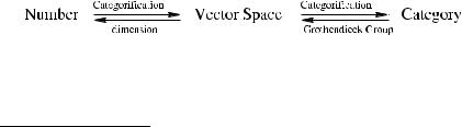
Topological ﬁeld theory is a natural framework for “categoriﬁcation”, an informal procedure that turns integers into vector spaces (Abelian groups), vector spaces into Abelian or triangulated categories, operators into functors between these categories [14]. The number becomes the dimension of the vector space, while the vector space becomes the Grothendieck group of the category (tensored with a ﬁeld). This procedure can be illustrated by the following diagram [29]: Recently, this idea led to

a number of remarkable developments in various branches of mathematics, notably in low-dimensional topology, where many polynomial knot invariants were lifted to homological invariants.

Sergei Gukov

Department of Physics, University of California, Santa Barbara, CA 93106, USA, e-mail: gukov@theory.caltech.edu

V. Sidoraviciusˇ (ed.), New Trends in Mathematical Physics,	313
© Springer Science + Business Media B.V. 2009

314	Sergei Gukov

Although the list of homological knot invariants is constantly growing, most of the existing knot homologies ﬁt into the “A-series” of homological knot invariants associated with the fundamental representation of sl(N ) (or gl(N )). Each such theory is a doubly graded knot homology whose graded Euler characteristic with respect to one of the gradings gives the corresponding knot invariant,

P (q) = (−1)i qj dim Hi,j .	(1)
i,j

For example, the Jones polynomial can be obtained in this way as the graded Euler characteristic of the Khovanov homology [37]. Similarly, the so-called knot Floer homology [62, 64] provides a categoriﬁcation of the Alexander polynomial Δ(q). At ﬁrst, these as well as other homological knot invariants listed in the table below appear to have very different character. Thus, as the name suggests, knot Floer homology is deﬁned as a symplectic Floer homology of two Lagrangian submanifolds in a certain conﬁguration space, while the other theories are deﬁned combinatorially. In addition, the deﬁnition of the knot Floer homology admits a generalization to knots in arbitrary 3-manifolds, whereas at present the deﬁnition of the other knot homologies (with N > 0) is known only for knots in R3.

Table 1 A general picture of knot polynomials and knot homologies

g	Knot Polynomial	Categoriﬁcation
gl(1\|1)	Δ(q)	knot Floer homology H F K(K)
“sl(1)”	–	Lee’s deformed theory H (K)
sl(2)	Jones	Khovanov homology H Kh(K)
sl(N )	PN (q)	sl(N ) homology H KRN (K)

The sl(N ) knot homology [37, 39, 41]—whose Euler characteristic is the quantum sl(N ) invariant PN (q)—has a physical interpretation as the space of BPS states, HBP S , in string theory [22]. In order to remind the physical setup of [22], let us recall that polynomial knot invariants, such as PN (q), can be related to open topological string amplitudes (“open Gromov-Witten invariants”) by ﬁrst embedding ChernSimons gauge theory in topological string theory [75], and then using the so-called large N duality [17, 18, 60, 49], a close cousin of the celebrated AdS/CFT duality [54]. Moreover, open topological string amplitudes and, hence, the corresponding knot invariants can be reformulated in terms of new integer invariants which capture the spectrum of BPS states in the string Hilbert space, HBP S . The BPS states in question are membranes ending on Lagrangian ﬁve-branes in M-theory on a noncompact Calabi-Yau space X = OP1 (−1) OP1 (−1). Speciﬁcally, the ﬁve-branes have world-volume R2,1 × LK where LK X is a Lagrangian submanifold (which depends on knot K) and R2,1 R4,1.

Surprisingly, the physical interpretation of the sl(N ) knot homology naturally leads to a triply-graded (rather than doubly-graded) knot homology [22] (see also

Surface Operators and Knot Homologies

315

Fig. 1 A membrane ending on a Lagrangian ﬁve-brane

[20, 23]). Indeed, the Hilbert space of BPS states, HBP S , is graded by three quantum numbers, which are easy to see in the physical setup described in the previous

=	×	SU (2)
paragraph. The world-volume of the ﬁve-brane breaks the SO(4) SU (2)		SU (2)

rotation symmetry in ﬁve dimensions down to a subgroup U (1)L × U (1)R , where U (1)L (resp. U (1)R ) is a rotation symmetry in the dimensions parallel (resp. transverse) to the ﬁve-brane. Therefore, BPS states in the effective N = 2 theory on the ﬁve-brane are labeled by three quantum numbers jL, jR , and Q, where

		=
Q		H2(X, LK ) Z is the relative homology class represented by the mem-

brane world-volume. In other words, apart from the Z2-grading by the fermion number, the Hilbert space of BPS states HBP S is triply-graded. The properties of this triply-graded theory were studied in [15]; it turns out that this theory uniﬁes all the doubly-graded knot homologies listed in Table 1, including the knot Floer homology. A mathematical deﬁnition of the triply-graded knot homology which appears to have many of the expected properties was constructed in [42].

Apart from realization in (topological) string theory, the homological knot invariants are expected to have a physical realization also in topological gauge theory, roughly as polynomial knot invariants have a physical realization in threedimensional gauge theory (namely, in the Chern-Simons theory [73]) as well as in the topological string theory [75, 17, 18, 60]. Although these two realizations are not unrelated, different properties of knot polynomials are easier to see in one description or the other. For example, the dependence on the rank N is manifest in the string theory description, while the skein operations and transformations under surgeries are easier to see in the Chern-Simons gauge theory.

Similarly, as we explained above, string theory realization is very useful for understanding relation between knot homologies of different rank. On the other hand, the formal properties of knot homologies which are hard to see in string theory (which, however, would be very natural in topological ﬁeld theory) have to do with the fact that, in most cases, knot homologies can be extended to a functor F from the category of 3-manifolds with links and cobordisms to the category of graded vector spaces and homomorphisms

316	Sergei Gukov
F (Y ; K) = HY ;K	(2)
F (X; D) : HY ;K → HY ;K	(3)

Moreover, on manifolds with corners, it is expected that F extends to a 2-functor from the 2-category of oriented and decorated 4-manifolds with corners to the 2- category of triangulated categories [38, 34, 2]. In particular, it should associate:

•A triangulated category F (Σ) to a closed oriented 2-manifold Σ ;

•An exact functor F (Y ) to a 3-dimensional oriented cobordism Y ;

•A natural transformation F (X) to a 4-dimensional oriented cobordism X.

As we explain below, these are precisely the formal properties of a four—dimen- sional topological ﬁeld theory with boundaries and corners. Moreover, links and link cobordisms can be incorporated by introducing “surface operators” in the topological gauge theory.

In Sect. 2, we discuss the general aspects of topological gauge theories which admit surface operators. Of particular importance is the fact that every topological gauge theory which admits surface operators gives rise to an action of the braid group on D-branes. Then, in Sects. 3 and 4 we illustrate how these general structures are realized in simple examples of N = 2 and N = 4 twisted gauge theories. Speciﬁcally, in Sect. 3 we study surface operators and the corresponding knot homologies in the Donaldson-Witten theory and in the Seiberg-Witten theory, both of which are obtained by twisting N = 2 supersymmetric gauge theory. In Sect. 4, we explain that a particular twist of the N = 4 super-Yang-Mills theory—studied recently in connection with the geometric Langlands program [36, 21]—with a simple type of surface operators provides a physical framework for categoriﬁcation of the GC Casson invariant.

2 Gauge Theory and Categoriﬁcation

Let us start by describing the general properties of the topological quantum ﬁeld theory (TQFT) with boundaries, corners, and surface operators. To a closed 4-manifold

X, a four-dimensional TQFT associates a number, Z(X), the partition function of the topological theory on X. Similarly, to a closed 3-manifold Y , it associates a vector space, HY , the Hilbert space obtained by quantization of the theory on

X= R × Y . Finally, to a closed surface Σ it associates a triangulated category, F (Σ), which can be understood as the category of D-branes in the topological sigma-model obtained via the dimensional reduction of gauge theory on Σ . The objects of the category F (Σ ) describe BRST-invariant boundary conditions in the

four-dimensional TQFT on 4-manifolds with corners (locally, such manifolds look like X = R × R+ × Σ ). Summarizing,

gauge theory on X gauge theory on R × Y gauge theory on R2 × Σ

number Z(X)

vector space HY

category F (Σ )

Surface Operators and Knot Homologies

317

where we assume that X, Y , and Σ are closed. Depending on whether the topological reduction of the four-dimensional gauge theory on R2 × Σ gives a topological A-model or B-model, the category F (Σ ) is either the derived Fukaya category,1 Fuk(M ), or the derived category of coherent sheaves, Db(M ) := DbCoh(M ),

topological A-model:			F (Σ) =	Fuk(			M	)
				D	b
topological B-model: F (Σ) =						(M )
where M is the moduli space of	classical solutions in gauge theory on R2								× Σ ,
	2
invariant under translations along R		. Different topological gauge theories lead to

different functors F . For example, in the context of Donaldson-Witten theory [72], Fukaya suggested [16] that the category associated to a closed surface Σ should be A∞-category of Lagrangian submanifolds in the moduli space of ﬂat G-connections on Σ . This is precisely what one ﬁnds from the topological reduction [3] of the twisted N = 2 gauge theory on R2 × Σ, in agreement with the general principle discussed here.

The Atiyah-Floer Conjecture and Its Variants

It is easy to see that F deﬁned by the topological gauge theory has all the expected properties of a 2-functor. In particular, to a 3-manifold Y with boundary ∂Y = Σ it associates a “D-brane”, that is an object in the category F (Σ ).

Fig. 2 (a) A 3-manifold Y can be obtained as a connected sum of 3-manifolds Y1 and Y2, joined along their common boundary Σ. (b) In four-dimensional gauge theory, the space R×Y is obtained by gluing two 4-manifolds with corners

The interpretation of 3-manifolds with boundary as D-branes can be used to reproduce the Atiyah-Floer conjecture, which states [1]:

H F inst	(Y ) H F symp		(M	;	L1, L2)	(4)
	=			;

Here M = MﬂatG is the moduli space of ﬂat connections on Σ , while L1 and L2 are Lagrangian submanifolds in M associated with the Heegard splitting of Y ,

Y = Y1 Σ Y2

(5)

1 Notice, according to the Homological Mirror Symmetry conjecture, this category is equivalent to the derived category of the mirror B-model [44]. In particular, the category Fuk(M ), suitably deﬁned, must be a triangulated category [7].

318	Sergei Gukov
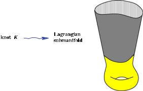
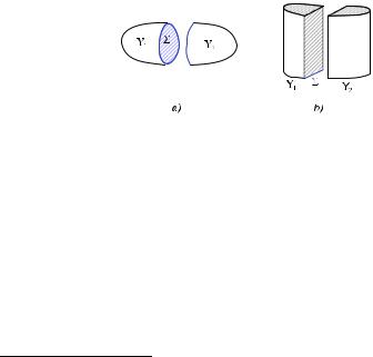
such that the points of Li	M , i = 1, 2, correspond to ﬂat connections on Σ

which can be extended to Yi .

Similarly, in the B-model, Y1 and Y2 deﬁne the corresponding B-branes, which are objects in the derived category of coherent sheaves on M . In both cases, the vector space HY associated with the compact 3-manifold Y is the space of “1–2

strings”:	H F symp(M ; L1, L2)
HY =	H F symp(M ; L1, L2)	A-model	(6)
HY =	Ext (FY1 , FY2 )	B-model

In the Donaldson-Witten theory, this leads to the Atiyah-Floer conjecture (4).

“Decategoriﬁcation”

The operation represented by the arrow going to the left in (1)—“decategoriﬁc- ation”—also has a natural interpretation in gauge theory. It corresponds to the dimensional reduction, or compactiﬁcation on a circle. Indeed, the partition function in gauge theory on X = S1 × Y is the trace (the index) over the Hilbert space HY :

ZS1×Y = χ (HY )

(7)

Similarly, the vector space associated with Y = S1 × Σ is the Grothendieck group of the category F (Σ )

	HS1×Σ = K(F (Σ))		(8)
In the case of A-model and B-model, respectively, we ﬁnd
K(F (Σ )) =	H d (M )	for F (Σ ) = Fuk(M )	(9)
	H (M )	for F (Σ ) = Db(M )

where d = 12 dim(M ).

2.1 Incorporating Surface Operators

In a three-dimensional TQFT, knots and links can be incorporated by introducing topological loop observables. The familiar example is the Wilson loop observable in Chern-Simons theory,

WR (K) = TrR P exp A (10)

Recall, that canonical quantization of the Chern-Simons theory on Σ × R associates a vector space HΣ —the “physical Hilbert space”—to a Riemann surface Σ [73]. In presence of Wilson lines, quantization gives a Hilbert space HΣ ;pi ,Ri canonically associated to a Riemann surface Σ together with marked points pi (points where Wilson lines meet Σ) decorated by representations Ri . For example, to n

Surface Operators and Knot Homologies

319

marked points on the plane colored by the fundamental representation it associates V n, where V is a N -dimensional irreducible representation of the quantum group

Uq (sl(N )).

We wish to lift this to a four-dimensional gauge theory by including the “time” direction, so that the space-time becomes X = Y × R, where the knot K is represented by a topological defect (which was called a “surface operator” in [21]) localized on the surface D = K × R. In the Feynman path integral, a surface operator is deﬁned by requiring the gauge ﬁeld A (and perhaps other ﬁelds as well) to have a prescribed singularity. For example, the simplest type of singularity studied in [21] creates a holonomy of the gauge ﬁeld on a small loop around D,

V = Hol(A)

(11)

Quantization of the four-dimensional topological theory on a 4-manifold X = Y ×R with a surface operator on D = K × R gives rise to a functor that associates to this data (namely, a 3-manifold Y , a knot K, and parameters of the surface operator) a vector space, the space of quantum ground states,

F (Y ; K) = HY ;K,parameters

(12)

Moreover, we will be interested in surface operators which preserve topological invariance for more general 4-manifolds X and embedded surfaces D X. For example, if the four-dimensional topological gauge theory is obtained by a topological twist of a supersymmetric gauge theory, it is natural to consider a special class of surface operators which preserve supersymmetry, in particular, those supercharges which become BRST charges in the twisted theory. Such surface operators can be deﬁned on a more general embedded surface D, which might be either closed or end on the boundary of X. An example of this situation is a four-dimensional TQFT with corners, shown on Fig. 3, which arises when we consider a lift of a 3-manifold with boundary Σ and line operators with end-points on Σ.

To summarize, including topological surface operators in the four-dimensional gauge theory, we obtain a functor from the category of 3-manifolds with links and their cobordisms to the category of graded vector spaces and homomorphisms:

Fig. 3 (a) Line operators in a three-dimensional TQFT on Σ × I and (b) topological “surface operators” in four-dimensional gauge theory on Σ × I × R

320	Sergei Gukov
F (X; D) : HY ;K → HY ;K	(13)

Here, the knot homology HY ;K is the space of quantum ground states in the fourdimensional gauge theory with surface operators and boundaries. Similarly, the functor F associates a number (the partition function) to a closed 4-manifold with embedded surfaces, and a category F (Σ; pi ) to a surface Σ with marked points, pi , which correspond to the end-points of the topological surface operators.

As in the theory without surface operators, the category F (Σ ; pi ) is either the category of A-branes or the category of B-branes on M , depending on whether the topological reduction of the four-dimensional gauge theory is A-model or B- model. Here, M is the moduli space of R2-invariant solutions in gauge theory on X = R2 × Σ with surface operators supported at R2 × pi .

2.2 Braid Group Actions

As we just explained, surface operators are the key ingredients for realizing knot homologies in four-dimensional gauge theory. Our next goal is to explain that every topological gauge theory which admits surface operators is, in a sense, a factory that produces examples of braid group actions on branes, including some of the known examples as well as the new ones.2

In general, the mapping class group of the surface Σ acts on branes on M . In particular, when Σ is a plane with n punctures, the moduli space M is ﬁbered over the conﬁguration space Confn(C) of n unordered points on C,

M
↓n	(14)
Conf (C)

and the braid group Brn = π1(Confn(C)) (= the mapping class group of the n- punctured disk) acts on the category F (Σ). Recall, that the braid group on n strands, Brn, has n − 1 generators, σi , i = 1, . . . , n − 1 which satisfy the following relations

σi σi+1σi = σi+1σi σi+1	(15)
σi σj = σj σi , \|i − j \| > 1	(16)

where σi can be represented by a braid with only one crossing between the strands i and i + 1, as shown on the ﬁgure below.

In gauge theory, the action of the braid group on branes is induced by braiding of the surface operators. Namely, a braid, such as the one on Fig. 4, corresponds

2 It is worth pointing out that, compared to [21], where the braid group action is associated with local singularities in the moduli space M , in the present context the origin of the braid group action is associated with global singularities.

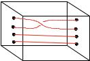
Surface Operators and Knot Homologies

321

Fig. 4 A braid on four strands

to a non-contractible loop in the conﬁguration space, Confn(C). As we go around the loop, the ﬁbration (14) has a monodromy, which acts on the category of branes F (Σ) as an autoequivalence,

Brn → Auteq(F (Σ ))	(17)
β → φβ	(18)

The simplest situation where one ﬁnds the action of the braid group Brn on A-branes (resp. B-branes) on M is when M contains An−1 chain of Lagrangian spheres (resp. spherical objects).

We remind that an An−1 chain of Lagrangian spheres is a collection of Lagrangian spheres L1, . . . , Ln−1 M , such that

1	\|i − j \| = 1
#(Li ∩ Lj ) =	(19)
0	\|i − j \| > 1

These conﬁgurations occur when M can be degenerated into a manifold with singularity of type An−1. Indeed, to any Lagrangian sphere L M , one can associate a symplectic automorphism of M , the so-called generalized Dehn twist TL along L , which acts on H (M ) as the Picard-Lefschetz monodromy transformation

(TL ) (x) =	x − ([L ] · x)[L ]	if dim(x) = dim(L )	(20)
	x	otherwise

As shown in [68], Dehn twists TLi along An−1 chains of Lagrangian spheres satisfy the braid relations (15), and this induces an action of the braid group with n strands on the category of A-branes, Fuk(M ).

The mirror of this construction gives an example of the braid group action on B-branes [70]. In this case, the braid group is generated by the twist functors along spherical objects (“spherical B-branes”) which are mirror to the Lagrangian spheres. As the name suggests, an object E Db(M ) is called d-spherical if Ext (E , E ) is isomorphic to H (Sd , C) for some d > 0,

i	(E , E ) =	C	if i = 0 or d	(21)
Ext	(E , E ) =	0	otherwise	(21)

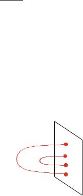
322	Sergei Gukov

A spherical B-brane deﬁnes a twist functor TE Auteq(Db(M )) which, for any F Db(M ), ﬁts into exact triangle

Hom (E , F ) E −→ F −→ TE (F )

(22)

where the ﬁrst map is evaluation. At the level of D-brane charges, the twist functor TE acts as, cf. (20),

x → x + (v(E ) · x) v(E )

where v(E ) = ch(E )√T d(M ) H (M ) is the D-brane charge (the Mukai vector) of E .

The mirror of an An−1 chain of Lagrangian spheres is an An−1 chain of spherical objects, that is a collection of spherical objects E1, . . . , En−1 which satisfy the condition analogous to (19),

dim Extk (Ei , Ej ) =	1	\|i − j \| = 1	(23)
k	0	\|i − j \| > 1

With some minor technical assumptions [70], the corresponding twist functors TEi generate an action of the braid group Brn on Db(M ). As we illustrate below, many examples of braid group actions on branes can be found by studying gauge theory with surface operators.

Fig. 5 A particular brane B which corresponds to closing a braid on four strands

In A-model as well as in B-model, the braid group action on branes can be used to write a convenient expression for knot homology, HK , of a knot K represented as a braid closure. Let K be a knot obtained by closing a braid β on both ends as shown on Fig. 5. Then, the space of quantum ground states, HK , in the four-dimensional gauge theory with a surface operator on D = R × K can be represented as the space of open string states between branes B and B = φβ (B). Here, B is the basic brane which corresponds to the conﬁguration on Fig. 5, while B is the brane obtained from it by applying the functor φβ ; it corresponds to the braid β closed on one side. These are A-branes (resp. B-branes) in the case of A-model (resp. B-

Surface Operators and Knot Homologies			323
model), and the space open strings is, cf. (6),
HK =	H F symp(M ; B, φβ (B))	A-model	(24)
HK =	Ext (B, φβ (B))	B-model

In particular, when topological reduction of the gauge theory gives A-model, the branes B and B are represented by Lagrangian submanifolds in M . This leads to a construction of link homologies via symplectic geometry, as in [69, 55, 56].

3Surface Operators and Knot Homologies in N = 2 Gauge

Theory

Now, let us illustrate the general structures discussed in the previous section in the context of N = 2 topological gauge theory in four dimensions. For simplicity, we consider examples of N = 2 gauge theories with gauge groups G = SU (2) and G = U (1) known as the Donaldson-Witten theory and the Seiberg-Witten theory, respectively. In fact, these two theories are closely related [67]—the former describes the low-energy physics of the latter—and below we shall use this fact to compare the corresponding knot homologies.

3.1 Donaldson-Witten Theory and the Equivariant Knot Signature

We start with pure N = 2 super-Yang-Mills theory with gauge group G which for simplicity we take to be SU (2). After the topological twist, the N = 2 gauge theory can be formulated on arbitrary 4-manifold X and localizes on the anti-self- dual (“instanton”) ﬁeld conﬁgurations [72]:

FA+ = 0

(25)

The space of quantum ground states on R × Y is the instanton Floer homology deﬁned3 by studying the gradient ﬂow of the Chern-Simons functional,


			HY = H F inst(Y )		(26)
and the topological	reduction [3] on R2			× Σ leads to a topological A-model with
		G
the target space M =		Mﬂat	, the moduli space of ﬂat connections on Σ. As we

already mentioned in the previous section these facts, together with the interpretation of boundaries as D-branes, naturally lead to the statement of the Atiyah-Floer conjecture. The Euler characteristic of HY is the Casson invariant, λG(Y ), which

3 As in the original Floer’s deﬁnition, we mainly assume that Y is a homology sphere when we talk about H F inst(Y ) in order to avoid difﬁculties related to reducible connections.

324 Sergei Gukov

computes the Euler characteristic of the moduli space of ﬂat G-connections on Y ,

χ (HY ) = 4λG(Y )

(27)

In the special case of G = SU (2) that we are mainly considering here, it is the standard Casson-Walker-Lescop invariant λCW L(Y ) which sometimes we write simply as λ(Y ).

We note that, while the homological invariant HY is difﬁcult to study on 3- manifolds with b1 > 1, its Euler characteristic—which is, at least formally, computed by the partition function of the four-dimensional gauge theory on X = S1 × Y —is still given by the Casson invariant [57],

ZDW (S1 × Y ) = 4λ

(28)

Since b2+(X) = b1(Y ) for X = S1 × Y , computing (28) is much easier in the case b1(Y ) > 1. Indeed, in general the Donaldson-Witten partition function ZDW (X) can be written as a sum of the contribution of the Coulomb branch (the u-plane integral) and two contributions, ZM and ZD , both of which are described by the Seiberg-Witten theory (that we consider in more detail below):

ZDW = Zu + ZM + ZD

(29)

For manifolds X = S1 × Y with b1(Y ) > 1 the u-plane integral vanishes and we have ZM = ZD = 2λ(Y ), which then add up to (27). If b1(Y ) = 1, the DonaldsonWitten partition function ZDW (S1×Y ) depends on the metric. In particular, it should be compared with the Euler characteristic of HY in the chamber R → ∞, where R is the radius of S1. In this case, the u-plane integral is non-zero, and instead of (28) one ﬁnds a similar expression with the “correction” − 46 |TorH1(Y, Z)|, see [57] for more details.

Surface Operators

Now let us consider surface operators in the Donaldson-Witten theory which correspond to the singularity of the gauge ﬁeld of the form

A = αdθ + · · ·

(30)

Here, (r, θ ) are radial coordinates in the normal plane, α is the parameter which labels surface operators and takes values in t = Lie(T), the Lie algebra of the maximal torus T G, and the dots in (30) stand for less singular terms. More precisely, inequivalent choices of α are labeled by elements in T = t/Λcochar since gauge transformations shift α by vectors in the cocharacter lattice Λcochar of G. For example, for G = SU (2) we have T = U (1).

In the presence of a surface operator on D X, supersymmetric ﬁeld conﬁgurations in this theory are described by the instanton equations (25):

FA+ = 2π α(δD )+

(31)

Surface Operators and Knot Homologies

325

perturbed by the term 2π α(δD )+, where (δD )+ denotes the self-dual part of the cohomology class that is Poincaré dual to the surface D. In the context of SU (2) gauge theory, such surface operators were extensively used in the work of Kronheimer and Mrowka on minimal genus problems of embedded surfaces in 4-manifolds [46, 47].

According to the general rules outlined in the previous section, to a 4-manifold X = R × Y and a surface operator on D = R × K labeled by e2π iα T the

Donaldson-Witten theory associates a vector space, the space of quantum ground states,

HY ;K,α = H F inst(Y ; K, α)

(32)

Just like the ordinary instanton Floer homology (27), it categoriﬁes a Casson-like invariant,

χ (HY ;K,α ) = λα (Y ; K)

(33)

which counts ﬂat SU (2) connections on a homology sphere Y with the prescribed singularity (30) along K.

	In order to describe λα (Y ; K) more explicitly, it is convenient to decompose Y as
				), and its complement,
in (5) into a tubular neighborhood of the knot K, Y1 = N (K2
	=		\	=	. As we already men-
Y2		Y		N (K), glued along the common boundary Σ T	. As we already men-

tioned earlier, topological reduction of the Donaldson-Witten theory on Σ yields a topological A-model with the target space M = MﬂatG , the moduli space of ﬂat connections on Σ :

MﬂatG = {ρ : π1(Σ ) → G}/conj.

(34)

For Σ = T 2 this moduli space is the quotient, MﬂatG = (T × T)/W , of two copies of the maximal torus by the Weyl group of G. In particular, for G = SU (2) the cor-

responding moduli space G T 2/Z2 is often called the “pillowcase”. Similarly,

Mﬂat =

each component in the decomposition Y = Y1 Σ Y2 deﬁnes an A-brane supported on a Lagrangian submanifold in MﬂatG . If we denote Lagrangian submanifolds associated to Y1 and Y2, respectively, by Lα and LY \K , then the invariant (33) is given by their intersection number (in the smooth part of MﬂatG ):

λα (Y ; K) = #(Lα ∩ LY \K )

(35)

Note, the Lagrangian brane supported on Lα does not depend on K or Y , while the Lagrangian brane supported on LY \K does not depend on α. Indeed, Lα is simply the set of representations ρ MﬂatG taking the meridian of the knot K to a matrix of trace tr(ρμ) = 2 cos π α. Similarly, the Lagrangian brane supported on LY \K corresponds to ﬂat connections on Σ = T 2 which can be extended to ﬂat connections

on Y \ K. In other words, LY \K is the image of MﬂatG (Y \ K) under the restriction map

r : MﬂatG (Y \ K) → MﬂatG (T 2)

induced by the inclusion of the torus boundary of the knot complement, T 2 → Y \ K.

326 Sergei Gukov

To summarize, surface operators in the Donaldson-Witten theory lead to a variant of the instanton Floer homology, HY ;K.α , whose Euler characteristic is a Cassonlike invariant (35). This is precisely the deﬁnition of the knot invariant which was introduced and studied in [53, 9, 25] (see also [26, 45]). This invariant, sometimes called Casson-Lin invariant, is well-deﬁned away from the roots of the Alexander polynomial of K and turns out to be equal to the linear combination of more familiar

invariants, α [0, 1],
λα (Y ; K) = 4λ(Y ) +	1	σα (K)	(36)

	2

where λ(Y ) is the Casson invariant of Y and σα (K) : U (1) → Z is the equivariant signature function (a.k.a. Levine-Tristram signature) of the knot K. Homology theory categorifying λα (Y ; K) was constructed in [12] (see also [10, 11]) and, therefore, is expected to be the same as (32).

We remind that, for a knot K in a homology sphere Y , the normalized Alexander

polynomial is deﬁned as
Δ(K; q) = det q1/2V − q−1/2VT	(37)

where V is the Seifert matrix of K The equivariant signature σα (K)

and q = e2π iα . Note, that Δ(K; q) = Δ(K; q−1). is deﬁned as the signature of the Hermitian matrix

BK (q) = (1 − q)V + (1 −

q)VT

(38)

The equivariant signature function changes its value only if q = e2π iα is a root of the Alexander polynomial. It vanishes for α near 0 or 1,

α	lim		σα (K) = 0	(39)
	→	0,1

and equals the standard knot signature, σ (K), for α = 12 . In particular, for Y = S3

and α = 12 we get the original Lin’s invariant [53] and the corresponding homol-

ogy theory categorifying λ 1 (Y ; K) was constructed—as symplectic Floer homol-

ogy (24) of the braid representative of K—in [50].

3.2 Seiberg-Witten Theory

Now let us consider N = 2 twisted gauge theory with Abelian gauge group G = U (1) coupled to a single monopole ﬁeld M. This theory localizes on the solutions to the Seiberg-Witten equations for Abelian monopoles [74]:

	M)+ = 0
FA+ + i(M		(40)
D/AM = 0		(41)

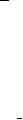
Surface Operators and Knot Homologies

327

which follow from the N = 2 topological gauge theory.4 The partition function of this theory on a 4-manifold X with 2-observables included is a generating function of the Seiberg-Witten invariants, SWX (x), which “count” solutions to (40) and can be viewed as a function of x Spinc(X),

SWX : Spinc(X) → Z

To be more precise, the Seiberg-Witten invariants are deﬁned as integrals over Mx , the moduli space of solutions to the Seiberg-Witten equations (40),

SWX (x) = aDdx /2

where dx = 14 (x2 − 2χ (X) − 3σ (X)) is the virtual dimension of Mx , and aD is a 2-form which represents the ﬁrst Chern class of the universal line bundle on the moduli space Mx .

The space of quantum ground states in this theory is the Seiberg-Witten mono-

pole homology,
HY = H M (Y )	(44)

which is conjectured to be isomorphic to the Heegard Floer homology, see e.g. [48]:

	=		(Y )	(45)
H M	(Y ) H F

In turn, the Heegard Floer homology H F (Y )—as well as its analog for knots, the knot Floer homology H F K (K), that is closer to our interest—is deﬁned as the symplectic Floer homology of certain Lagrangian submanifolds in the symmetric product space of the form [62, 64, 61],

M = Symk (Σ)

(46)

The symmetric product space and Lagrangian submanifolds in it naturally appear in the topological reduction of the Seiberg-Witten theory. Indeed, on X = R2 × Σ the

4 Up to the ﬁnite group H 1(X, Z2), the set of Spinc structures on a 4-manifold X is parameterized by integral cohomology classes which reduce to w2(X) mod 2,

Spinc (X) = {x H 2(X, Z) | x ≡ w2(X) mod 2}

Given a Spinc structure x Spinc (X), let L be the corresponding Hermitian line bundle, and SL± the corresponding spinor bundles. Then, the Seiberg-Witten monopole equations (40) are equations for a pair (A, M), where A is a unitary connection on L and M is a smooth section of SL+. In writing the equations (40) we used the Dirac operator,D/A : SL+ → SL−, and a map

		Ω0(SL+) →	Ω0(ad0SL+)	(42)
		M →		(43)
		M →	i(MM)+	(43)
=	+
where ad0SL+	Λ2	is the subbundle of the adjoint bundle of SL+ consisting of the traceless skew-

Hermitian endomorphisms, which can be identiﬁcation with the space of self-dual 2-forms.

328	Sergei Gukov

equations (40) reduce to the vortex equations in the Abelian Higgs model, and the moduli space of solutions to these equations, namely the moduli space of charge k vortices, is the symmetric product space (46), see [35]. As in the case of the Donaldson-Witten theory, the topological reduction of the Seiberg-Witten theory leads to the topological A-model5 with M as the target space, and the corresponding category of branes in this case is the category of A-branes,

F (Σ ) = Fuk(M )

(47)

According to the general rules explained in the previous section, the Euler characteristic of the homology theory (44), (45) is given by the partition function of the

Seiberg-Witten theory on X = S1 × Y (in the chamber R → ∞):
ZSW (Y ) =	SWY (x)	(48)
	x Spinc (Y )

If b1(Y ) > 1, then there are no wall-crossing phenomena and ZSW (Y ) can be equivalently viewed as the partition function of the three-dimensional gauge theory on Y obtained by the dimensional reduction of the Seiberg-Witten theory. For a fairly general class of 3-manifolds Y , the partition function (48) is equal to the Casson invariant of Y , cf. (28):

ZSW (Y ) = λ(Y )

(49)

For instance, for 3-manifolds with b1(Y ) > 1 it follows e.g. from the general result of Meng and Taubes [58] that will be discussed in more detail below. On the other hand, for homology spheres the deﬁnition of the Seiberg-Witten invariants requires extra care. However, once this is done, one can show that (49) still holds for suitably deﬁned ZSW (Y ); see [52, 8, 59] for a mathematical proof and [4] for a physical argument based on the duality with Rozansky-Witten theory [65].

Surface Operators

As in the Donaldson-Witten theory, we can introduce surface operators by requiring the gauge ﬁeld to have the singularity of the form (30). In the Seiberg-Witten theory, such surface operators are labeled by e2π iα U (1). In the presence of a surface operator on D X, supersymmetric ﬁeld conﬁgurations are described by the perturbed Seiberg-Witten monopole equations, cf. [74, 71]:

	M)+ = 2π α(δD )+
FA+ + i(M		(50)
D/AM = 0		(51)

As usual, in order to obtain a homological invariant of a knot K in a 3-manifold Y0 one should consider the Hilbert space of the gauge theory on X = R × Y0 with a surface operator on D = R × K. In the context of Seiberg-Witten theory, this gives a vector space HY0;K;x,α . More generally, given a link L with components one

5 In fact, this is true for any four-dimensional N = 2 gauge theory with the same type of topological twist [3].

Surface Operators and Knot Homologies

329

can introduce surface operators, each with its own parameter αi , i = 1, . . . , . The corresponding Hilbert space is

HY0;L;xi ,αi = H M (Y ; xi , αi )

(52)

where Y = Y0 \L is the link complement, and parameters αi determine the boundary conditions on Y . Namely, the holonomy of the U (1) gauge connection A along the meridian of the i-th link component should be equal to e2π iαi . We will be mainly interested in the case where Y0 = S3 and Y = S3 \ L is the link complement. In this case, (52) gives ( + 1)-graded link homology.

We introduce the graded Euler characteristic of the homological invariant (52),

ταi (Y ; qi ) :=			χ (H M (Y ; xi , αi )) · qx								(53)
		x H (Y )
which is a formal power series in q±1			, where q	i	=	ehi and h			are the generators of
a free Abelian group,		i		i	=			i
a free Abelian group,
H (Y )	:=	H1(Y, Z)/torsion Zb1(Y )
	:=				=				=		=
In particular, when Y is a link complement, the group H (Y )									=		=
										H1	(Y, Z) Z is
generated by the meridians of the link components.
In general, ταi (Y ; qi ) is a non-trivial function of qi							and		αi . It is equal to the
In general, ταi (Y ; qi ) is a non-trivial function of qi							S	1	αi . It is equal to the
partition function of the Seiberg-Witten theory on X =							S		× Y (in the chamber
R → ∞):			SWY (x, αi ) · qx
ταi (Y ; qi ) =			SWY (x, αi ) · qx								(54)

x H (Y )

This function is an interesting generalization of the Reidemeister-Milnor torsion, on the one hand, and the equivariant knot signature, on the other. Indeed, since the Seiberg-Witten theory is the low-energy description of the Donaldson-Witten theory, we expect the relation to the equivariant knot signature. On the other hand, if αi is near 0 or 1 for all i = 1, . . . , , as in (39), then the partition function ZSW (Y ; xi , αi ) = ταi (Y ; qi ) becomes the ordinary partition function of the link complement Y studied by Meng and Taubes [58] who showed that it is equal to the Reidemeister-Milnor torsion. Hence,

αi

lim

αi

;

)

τ (Y

;

)

(55)

0,1

→

where τ (Y ; qi ) is the ordinary Reidemeister-Milnor torsion of Y . In particular, for b1(Y ) > 1 we have τ (Y ; qi ) = Δ(L; qi ), so that in this limit the homological invariant (52) categoriﬁes the multi-variable Alexander polynomial Δ(L; qi ) of the link L,

χ (HL;x ) · qx = Δ(L; q)

(56)

x H (Y )

330 Sergei Gukov

This suggests to identify the ( + 1)-graded homology theory (52) with the link Floer homology [63],

HL;x = H F L (L; x)

(57)

In the case of knots, the relation to the Alexander polynomial Δ(K; q) is slightly more delicate, in part due to metric dependence and wall crossing. It turns out, however, that even though individual Seiberg-Witten invariants are different in the positive and negative chamber, the corresponding generating functions are both equal to the Milnor torsion [58], so that (55) still holds. Note, that specializing (55) further to qi = 1, we recover (49). It would be interesting to study the invariant τα (Y ; q) further, in particular, its relation to the equivariant knot signature σα (K).

4Surface Operators and Knot Homologies in N = 4 Gauge

Theory

Now, let us consider surface operators and knot homologies in the context of N = 4 topological super-Yang-Mills theory in four dimensions. Speciﬁcally, we shall consider the GL twist of the theory [36], with surface operators labeled by regular semisimple conjugacy classes [21]. As we shall explain below, this theory provides a natural framework for categoriﬁcation of the GC Casson invariant, which counts ﬂat connections of the complexiﬁed gauge group GC.

The topological reduction of this theory leads to a N = 4 sigma-model [3, 24, 36], whose target space is a hyper-Kahler manifold MH (Σ, G), the moduli space

of solutions to the Hitchin equations on Σ [27]:
F − φ φ = 0	(58)
dAφ = 0, dA φ = 0	(59)

This twist of the N = 4 super-Yang-Mills theory has a rich spectrum of supersymmetric surface operators. In particular, here we will be interested in the most basic type of surface operators, which correspond to the singular behavior of the

gauge ﬁeld A and the Higgs ﬁeld φ of the form [21]:
A = αdθ + · · · ,				(60)
dr
φ = β		− γ dθ	+ · · ·	(61)
	r

where α, β, γ t, and the dots stand for the terms less singular at r = 0. For generic values of the parameters α, β, γ , (60) deﬁnes a surface operator associated with the regular semi-simple conjugacy class C GC.

According to the general rules explained in Sect. 2, this topological ﬁeld theory associates a homological invariant HY to a closed 3-manifold Y and, more generally, a knot homology HY ;K to a 3-manifold with a knot (link) K. These homologies can be computed as in (6) and (24) using the Heegard decomposition of Y as

Surface Operators and Knot Homologies

331

well as the braid group action on branes. The branes in questions6 are branes of type (A, B, A) with respect to the three complex structures (I, J, K) of the hyper-Kahler space MH (Σ, G). We can use this fact and analyze the branes in different complex structures in order to gain a better understanding of the homological invariant HY,K as well as the GC Casson invariant itself. For example, in complex structure I it corresponds to counting parabolic Higgs bundles, a fact that has already been used e.g. in [5] for studying the SL(2, C) Casson invariant for Seifert ﬁbered homology spheres.

Complex Structure J : Counting Flat Connections

The B-model in complex structure J is obtained, e.g. by setting the theta angle to zero, Re(τ ) = 0, and choosing t = i (where t is a complex parameter that labels a family of GL twists of the N = 4 super-Yang-Mills [36]). In complex

structure J , the moduli space H (Σ, G) GC (Σ ) is the space of complexiﬁed

M = Mﬂat

ﬂat connections A = A + iφ, and the surface operator (60) creates a holonomy,

V = Hol(A ),

which is conjugate to exp(−2π(α − iγ )). Furthermore, at t = i the supersymmetry equations of the four-dimensional gauge theory are equivalent to the ﬂatness equations, dA + A A = 0, which explains why (from the viewpoint of complex structure J ) the partition function of this theory on X = S1 × Y with a surface operator on D = S1 × K computes the GC Casson invariant,

Z = λGC (Y ; K)

The space of ground states, HY ;K , is a categoriﬁcation of λGC (Y ; K). In general, both λGC (Y ; K) and HY ;K depend on the holonomy V , which characterizes surface operators. However, if V is regular semi-simple, as we consider here, then λGC (Y ; K) and HY ;K do not depend on a particular choice of V .

Complex Structure K

Since the four-dimensional topological gauge theory (even with surface operators) does not depend on the parameter t that labels different twists, we can take t = 1, which leads to the A-model on MH (Σ, G) with symplectic structure ωK . This theory computes the same GC Casson invariant and its categoriﬁcation, HY ;K ,

but via counting solutions to the following equations on Y [36]:
F − φ φ = Dφ0 − [A0, φ]	(62)
Dφ = [φ0, φ] + DA0	(63)
D φ + [A0, φ0] = 0	(64)

rather than ﬂat GC connections. In particular, given a Heegard decomposition Y = Y1 Σ Y2, the space of solutions to (62) on Y1 (resp. Y2) deﬁnes a Lagrangian

6 E.g. branes B1 and B2 associated with the Heegard decomposition Y = Y1 Σ Y2.

332 Sergei Gukov

A-brane in MH (Σ, G) with respect to ωK . This allows to express HY ;K as the space of open string states between the corresponding A-branes B1 and B2, cf. (6),

HY ;K = H F symp(MH ; B1, B2)

This alternative deﬁnition of the GC Casson invariant and its categoriﬁcation that follows from the twisted N = 4 gauge theory can be useful, for instance, for understanding situations when the (A, B, A) branes B1 and B2 intersect at singular points in MH or over higher-dimensional subvarieties.

Categoriﬁcation of the SL(2, C) Casson Invariant

Now, let us return to the complex structure J and, for simplicity, take the gauge group to be G = SU (2). Furthermore, we shall consider an important example of the sphere with four punctures:

Σ = CP1 \ {p1, p2, p3, p4}

which in gauge theory corresponds to inserting four surface operators. In complex structure J , MH (Σ, G) is the moduli space of ﬂat GC = SL(2, C) connections with ﬁxed conjugacy class of the monodromy around each puncture. It can be identiﬁed with the space of conjugacy classes of monodromy representations

{

π1

(Σ )

→

ρ(γi )

}

MH (Σ, G)

where the representations are restricted to take the simple loop γi around the i-th puncture into the conjugacy class Ci GC.

Using the fact that π1(Σ) is free on three generators, we can explicitly describe the moduli space MH (Σ, G) by introducing holonomies of the ﬂat SL(2, C) connection around each puncture,

Vi = Holpi (A ), i = 1, . . . , 4

(65)

where V1V2V3V4 = 1 and each Vi is in a ﬁxed conjugacy class. Following [32, 30, 33, 66, 28], we introduce the local monodromy data

Fig. 6 Sphere with four punctures

Surface Operators and Knot Homologies	333
trVi	i = 1, 2, 3
ai =	(66)

tr(V3V2V1) i = 4

and

θ1 = a1a4 + a2a3 θ2 = a2a4 + a1a3 θ3 = a3a4 + a2a1

(67)

(68)

θ4 = a1a2a3a4 + ai2 − 4	(69)
i=1

which determines the conjugacy classes of Vi . We also introduce the variables

x1	= tr(V3V2)	(70)
x2	= tr(V1V3)	(71)
x3	= tr(V2V1)	(72)

which will be the coordinates on the moduli space MH (Σ, G). Namely, the moduli space we are interested in is

MH (Σ, G) = {(V1, . . . , V4) | Vi Ci , V1V2V3V4 = 1}/GC

In terms of the variables (70), it can be explicitly described as the afﬁne cubic

MH (Σ, G) = {(x1, x2, x3) C3 \| f (xi , θm) = 0}	(73)
where
3
f (xi , θm) = x1x2x3 + (xi2 − θi xi ) + θ4	(74)
i=1

Singularities in MH

For certain values of the monodromy data, the moduli space MH becomes singular. It is important to understand the nature of the singularities and when they develop. In fact, as we shall see below, interesting examples of branes pass through such singularities.

The discriminant Δ(f ) of the cubic (74) is a polynomial in ai of total degree 16 [31]:

		3	2	4
Δ(a) =	a4 +	i ai − (ai a4 − aj ak )		(ai2 − 4) (75)
1 2 3=1		i=1		i=1

where i = ±1. A special subfamily of cubics (74), which will play an important role in applications to knot invariants discussed below, corresponds to the case

= σi σj σi−1. Here and below we

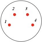
334 Sergei Gukov

where all monodromy parameters ai are equal, ai = a, i = 1, 2, 3, 4. In this case,

θi = 2a2, i = 1,	2, 3	(76)
θ4 = a4 + 4a2 − 4		(77)

and it is easy to verify that Δ(a) = 0. Speciﬁcally, for generic values of the parameter a, the moduli space MH has three simple singularities of type A1 (double points) at

(xi , xj , xk ) = (a2 − 2, 2, 2)

(78)

These singularities correspond to reducible ﬂat connections. For special values of a, the singularities can become worse and/or additional singularities can appear. For example, for a2 = 0 a new singularity of type A1 develops at the point (x1, x2, x3) = (−2, −2, −2). On the other hand, for a2 = 4 the moduli space has a simple singularity of type D4 at (x1, x2, x3) = (2, 2, 2).

Braid Group Action

The mapping class group of Σ , which in the present case is the braid group Br3, acts on the family of cubic surfaces (73) by polynomial automorphisms. In particular, one can verify that the generators σi , i = 1, 2, 3, represented as [32]:

σi : (xi , xj , xk , θi , θj , θk , θ4) → (θj − xj − xk xi , xi , xk , θj , θi , θk , θ4) (79)

satisfy the relations σi σj σi = σj σi σj and σk denote by (i, j, k) any cyclic permutation of (1, 2, 3).

Examples

Let us consider examples of (A, B, A) branes that arise from knotted surface operators in R × B3, where B3 denotes a 3-dimensional ball. We consider surface operators which are extended along the R direction and which meet the boundary S2 = ∂B3 at four points. The simplest example of such brane is

(80)

We shall denote this brane B (or B(14)(23) if we wish to specify which pairs of points on S2 it connects). Since the brane (80) identiﬁes the monodromies around the points 1 and 4 (resp. 2 and 3),

V1 = V4−1, V2 = V3−1

(81)

it can be explicitly described as a subvariety of MH deﬁned by

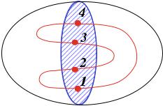
Surface Operators and Knot Homologies

335

	x1 = tr(V3V2) = 2	(82)
Of course, we also need to set a1 = a4 and a2 = a3, so that
θ1	= a12 + a22	(83)
θ2	= θ3 = 2a1a2	(84)
θ4	= a12a22 + 2a12 + 2a22 − 4	(85)

Substituting (82) and (83) into the cubic equation f (xi , θm) = 0, we ﬁnd that the brane (80) can be described as a degenerate quadric,

(x2 + x3 − a1a2)2 = 0

(86)

One can also think of it as a set of two coincident branes on x2 + x3 = a1a2. By acting on this brane with the elements of the braid group (79), we can construct other examples of (A, B, A) branes in MH . Furthermore, by closing the braid one can obtain homological invariants of knots (links) in S3 as spaces of open strings between two such branes. In the rest of this section, we consider a few explicit examples.

Unknot: One way to construct the unknot is to take surface operators which correspond to two branes of type (80), as shown on the ﬁgure below:

Fig. 7 Unknot in S3 can be represented as a union of two branes B

The two branes on this ﬁgure are branes B(14)(23) and B(12)(34). We already discussed the ﬁrst brane: it is described by the conditions (82)–(86). Similarly, the brane B(12)(34) is given by V1 = V2−1, which implies V3 = V4−1,

x3 = tr(V2V1) = 2

(87)

and the corresponding conditions for θi , cf. (83). Altogether, the conditions describing these two branes imply that the local monodromy data should be identiﬁed,

a1 = a2 = a3 = a4 = a

(88)

336	Sergei Gukov

This condition is very natural, of course, and will be relevant in all the examples where the resulting link has only one connected component, i.e. is actually a knot. Furthermore, for the unknot in Fig. 7 we have:

V1 = V2−1 = V3 = V4−1

(89)

These equations describe the intersection points of branes B(14)(23) and B(12)(34). Using (82) and (87), it is easy to see that there is only one such point (of multiplicity 2):

(x1, x2, x3) = (2, a2 − 2, 2)

(90)

This is precisely one of the singular points (78) where the moduli space MH has A1 singularity (for generic values of a) due to reducible representations. Therefore, we

conclude that the cohomology of the unknot, Hunknotsl(2) , is given by the space of open string states for two different branes intersecting at the A1 singularity in MH . We

point out that the values of xi in (90) can be read off directly from Fig. 7. Indeed, x1 = 2 simply follows from the fact that the combined monodromy around the points 2 and 3 is equal to the identity (similarly for x3 = 2). In order to explain x2 = a2 − 2, it is convenient to introduce the eigenvalues m±1 of the monodromy matrix V1. Of course, m is related to the local monodromy parameter a, namely a = m + m−1. Moreover, since V1 = V3, we have

x2 = tr(V1V3) = m2 + m−2 = a2 − 2

(91)

One can also construct the unknot using identical branes B and the braid group action on one of them:

Here, the two parts of the unknot correspond to the branes B and φσ1 (B), where B is the brane described in (80)–(86), and σ1 denotes the generator of the braid group Br3. Using the explicit form (79) of σ1, we ﬁnd that the brane φσ1 (B) is supported on the line:

Fig. 8 Unknot as a union of two branes B with a half-twist. Each vertical line represents a surface (topologically a 2-sphere) which divides S3 into two balls and meets the surface operator at four points

Surface Operators and Knot Homologies	337
φσ1 (B): x2 = 2	(92)

Together with (82), this condition implies that the branes B and φσ1 (B) meet only at one point (of multiplicity 2):

(x1, x2, x3) = (2, 2, a2 − 2)

(93)

which is precisely one of the A1 singularities (78) in the moduli space MH . This is in complete agreement with our previous analysis, where the same conﬁguration of D-branes in M was found starting from the presentation of the unknot shown on Fig. 7. This agreement was expected, of course, since both presentations of the unknot on Figs. 7 and 8 are homotopy equivalent in S3. The second presentation (on Fig. 8) can be easily generalized to the trefoil knot and more general torus knots (links) of type (2, k).

Trefoil Knot: The trefoil can be constructed by joining together the brane (80) and the brane obtained by action of three half-twists on B.

Starting with the equation (82) describing the brane B and applying σ1 three times, we ﬁnd that the brane φ(σ1)3 (B) is supported on the set of points

(x1, x2, x3) = (4z − 2a2z + 2a2z2 − 2z3 + y(1− z2), −2+ 2a2 − 2a2z + yz + 2z2, z)

(94)

where we assumed (88). Together with the equation f (xi ) = 0, this condition describes a subvariety in MH of complex dimension 1. Using (82) and (94), it is easy to see that the branes B and φ(σ1)3 (B) intersect at two points. The ﬁrst intersection point (of multiplicity 2) is precisely the singular point (93), as in the case of the unknot. The second intersection point (of multiplicity 4) is located at the regular point in MH ,

(x1, x2, x3) = (2, a2 − 1, 1)

(95)

Combining the contributions from the two intersection points, we ﬁnd that the cohomology for the trefoil knot has the following structure

Fig. 9 The trefoil knot in S3 can be represented as a union of two branes B with three half-twists

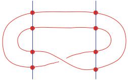
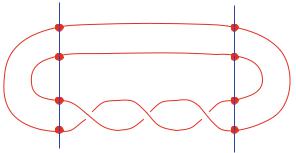
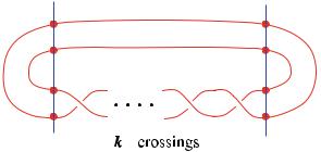
338			Sergei Gukov
sl(2)	sl(2)	sl(2)	(96)
Htrefoil	= Hunknot	H×	(96)

where Hunknotsl(2) is the contribution from the ﬁrst intersection point, and H×sl(2) denotes the contribution from the new intersection point (95). Discarding the contribu-

tion of reducible connections, we ﬁnd the reduced cohomology of the trefoil knot, which consists only of the term H×sl(2),

H×sl(2) = C4

(97)

Indeed, since MH is smooth near the intersection point, the conﬁguration of branes B and φ(σ1)3 (B) can be locally described (in complex structure J ) as an intersection of two sets of B-branes in C2, such that each set is supported on a line in C2. Let us consider a slightly more general problem where two sets of B-branes in C2 contain n1 and n2 branes, respectively. We denote by E1 and E2 the corresponding sheaves, where E1 (and similarly E2) is deﬁned by a module of the form C[x1, x2]/(xn1 ). The space of open string states between two such B-branes is given by

Ext	2 (E1, E2)	=	Cn1n2	(98)
C		=

which, of course, is the expected result since in the present case open strings form a hypermultiplet transforming in (n1, n2) under U (n1) × U (n2). Setting n1 = n2 = 2 gives (97).

(2, k) Torus Knots: A more general torus knot (link) T2,k can be represented as a union of two branes B with k half-twists.

In order to describe the action of (σ1)k on the brane (80), again we use (79). If the original brane B is represented by a set of two coincident branes on the line (cf. (86)),

(x1, x2, x3) = (2, y, a2 − y)

(99)

the result of (σ1)k action is a set of branes supported on a higher-degree curve

φ(σ1)k (B): (x1, x2, x3) = (Pk (y), Pk−1(y), a2 − y)

(100)

Fig. 10 The (2, k) torus knot (link) in S3 can be represented as a union of two branes B with k half-twists

= C4.

Surface Operators and Knot Homologies	339
where {Pi (y)}i≥−1 is a sequence of polynomials in y, such that	P0(y) = 2,
P−1(y) = y, and Pi (y), i > 1 are determined by the recursion relation
Pi (y) = 2a2 − (a2 − y)Pi−1(y) − Pi−2(y)
For example, the ﬁrst few polynomials Pi (y) look like
P1(y) = y	(101)
P2(y) = −2 + 2a2 − a2y + y2	(102)
P3(y) = 4a2 − 2a4 − 3y + 2a2y + a4y − 2a2y2 + y3	(103)
P4(y) = 2 − 4a4 + 2a6 + 8a2y − 4a4y − a6y − 4y2 + 2a2y2
+ 3a4y2 − 3a2y3 + y4	(104)
.
.	(105)
.	(105)

For simplicity, let us focus on torus knots, which correspond to odd values of k (the case of k even, which corresponds to torus links, can be treated similarly). Then, it

is easy to see that the brane φ(σ1)k (B) meets the brane (82) at (k + 1)/2 points in MH . As in the case of the trefoil knot, one intersection point (of multiplicity 2) is

the point (93) where MH has A1 singularity due to reducible connections. The other (k − 1)/2 points (each of multiplicity 4) are generically located at regular points in MH ; their precise location is determined by the explicit form of Pi (y). Therefore,

extending the earlier result (96), we ﬁnd that cohomology HTsl(2) of the torus knot

2,k

T2,k is isomorphic to a direct sum of Hunknotsl(2) and (k − 1)/2 copies of H×sl(2)

As usual, it is convenient to remove the contribution of reducible solutions. If we denote by HKsl(2) the “reduced” cohomology of K for the theory considered here, we can state our conclusion as

sl(2)	= 2(k − 1)
dim HT2,k	= 2(k − 1)	(106)

In general, the cohomology HKsl(2) categoriﬁes a variant of the Casson invariant obtained by counting ﬂat SL(2, C) connections on the knot complement S3 \ K with ﬁxed conjugacy class of the holonomy around the meridian,

χ (HKsl(2)) = 2σ (K)

(107)

We expect that, at least for a certain class of knots, σ (K) is the ordinary knot signature. Notice, that for (2, k) torus knots, we have σ (T2,k ) = (k − 1).

Finally, we note that one could obtain a different knot invariant (and, presumably, a different knot homology) by considering the image of the representation variety of the knot complement in the representation variety of the boundary torus, see e.g. [51]. Indeed, the boundary of the knot complement Y \ K can be identiﬁed with T 2 in the usual way, and the inclusion T 2 → Y \ K induces the restriction map

340								Sergei Gukov
GC		GC	2	)					(108)
r : Mﬂat	(Y \ K) → Mﬂat (T			)					(108)
which maps a representation ρ : π1(Y \K) → GC to its restriction ρ\|T 2								: π1(T 2) →
GC						GC	(T	2	) under the
GC. In general, Mﬂat (Y \K) is a branched cover of its image in Mﬂat							(T		) under the
restriction map (108). For example, if GC =		SL(2, C) and Y			=	S3	then, ignoring
restriction map (108). For example, if GC =				G	=
the multiplicity, the image of the representation variety MﬂatC (S3 \ K) under the
restriction map can be described as the zero locus7 of the A-polynomial [13],
	A(l, m) = 0								(109)

where the complex variables l and m parameterize, respectively, the conjugacy classes of the holonomy of the ﬂat SL(2, C) connection along the longitude and the meridian of the knot. The A-polynomial of every knot has a factor (l − 1) due to reducible representations. For example, the A-polynomial of a (2, k) torus knot looks like

A(T2,k ) = (l − 1)(lm2k + 1)

(110)

Notice, in this example, the part containing irreducible representations consists of a single curve, lm2k + 1 = 0, of degree one in l. On the other hand, the SL(2, C)

representation variety of T2,k is a cover of this curve by k−1 distinct irreducible

components which correspond to irreducible representations counted by N = 4 topological gauge theory. Restricting the complex variables l and m to be on a unit circle, we obtain the image of the SU (2) representation variety. For (2, k) torus knots, the SU (2) representation variety (again, ignoring reducible representations) is a disjoint union of k−2 1 nested open arcs [43, 6].

Acknowledgements I would like to thank N. Dunﬁeld, T. Hausel, A. Kapustin, M. Khovanov, M. Mariño, T. Mrowka, J. Roberts, and C. Vafa for clarifying discussions and comments. I am specially indebted to E. Witten for many useful discussions and for his observations on a preliminary version of this paper. This work is supported in part by DOE grant DE-FG03-92-ER40701, in part by RFBR grant 07-02-00645, and in part by the grant for support of scientiﬁc schools NSh-8004.2006.2.

This paper is an extended version of the talk delivered at the International Congress on Mathematical Physics 2006 (Rio de Janeiro) and at the RTN workshop “Constituents, Fundamental Forces and Symmetries of the Universe” (Napoli). I am very grateful to the organizers for the opportunity to participate in these meetings and to all the participants for providing a stimulating environment.

References

1. M.F. Atiyah, Floer homology. Prog. Math. Birkhauser 133, 105 (1995)

7 A-polynomial plays an important role in quantization of Chern-Simons theory with complex gauge group GC = SL(2, C), see [19].

Surface Operators and Knot Homologies

341

2.D. Bar-Natan, Khovanov’s homology for tangles and cobordisms. Geom. Topol. 9, 1443 (2005). math.GT/0410495

3.M. Bershadsky, A. Johansen, V. Sadov, and C. Vafa, Topological reduction of 4-d SYM to 2-d

sigma models. Nucl. Phys. B 448, 166 (1995). hep-th/9501096

4. M. Blau and G. Thompson, On the relationship between the Rozansky-Witten and the three-dimensional Seiberg-Witten invariants. Adv. Theor. Math. Phys. 5, 483 (2002). hep-th/0006244

5.H. Boden, and C. Curtis, The SL(2, C) Casson invariant for Seifert ﬁbered homology spheres and surgeries on twist knots. math.GT/0602023

6.H. Boden, C. Herald, P. Kirk, and E. Klassen, Gauge theoretic invariants of Dehn surgeries on knots. Geom. Topol. 5, 143 (2001). math.GT/9908020

7.A.I. Bondal and M.M. Kapranov, Framed triangulated categories. Math. USSR-Sb. 70, 93 (1991)

8.S. Cappell, R. Lee, and E. Miller, Surgery Formulae for Analytical Invariants of Manifolds. Contemp. Math., vol. 279. Am. Math. Soc., Providence (2001)

9.S. Cappell, R. Lee, and E. Miller, Equivariant Casson invariant. Preprint

10.O. Collin, Floer Homology for Orbifolds and Gauge Theory Knot Invariants, Knots, vol. 96, p. 201. Singapore, World Scientiﬁc (1997)

11.O. Collin, Floer homology for knots and SU (2)-representations for knot complements and cyclic branched covers. Can. J. Math. 52, 293 (2000)

12.O. Collin and B. Steer, Instanton Floer homology for knots via 3-orbifolds. J. Differ. Geom. 51, 149 (1999)

13.D. Cooper, M. Culler, H. Gillet, D.D. Long, and P.B. Shalen, Plane curves associated to character varieties of 3-manifolds. Invent. Math. 118, 47 (1994)

14.L. Crane and I. Frenkel, Four-dimensional topological quantum ﬁeld theory, Hopf categories, and the canonical bases. J. Math. Phys. 35, 5136 (1994). hep-th/9405183

15.N. Dunﬁeld, S. Gukov, and J. Rasmussen, The superpolynomial for knot homologies. Exp. Math. 15, 129 (2006). math.GT/0505662

16.K. Fukaya, Floer homology for 3-manifolds with boundary. In: Topology, Geometry, and Field Theory. World Scientiﬁc, River Edge (1994)

17.R. Gopakumar and C. Vafa, M-theory and topological strings. I. hep-th/9809187

18.R. Gopakumar, and C. Vafa, M-theory and topological strings. II. hep-th/9812127

19.S. Gukov, Three-dimensional quantum gravity, Chern-Simons theory, and the A-polynomial. Commun. Math. Phys. 255, 577 (2005). hep-th/0306165

20.S. Gukov and J. Walcher, Matrix factorizations and Kauffman homology. hep-th/0512298

21.S. Gukov and E. Witten, Gauge theory, ramiﬁcation, and the geometric Langlands program. hep-th/0612073

22.S. Gukov, A. Schwarz, and C. Vafa, Khovanov-Rozansky homology and topological strings. Lett. Math. Phys. 74, 53 (2005). hep-th/0412243

23.S. Gukov, A. Iqbal, C. Kozcaz, and C. Vafa, Link homologies and the reﬁned topological vertex. arXiv:0705.1368

24.J. Harvey, G. Moore, and A. Strominger, Reducing S duality to T duality. Phys. Rev. D 52, 7161 (1995). hep-th/9501022

25.C. Herald, Existence of irreducible representations of knot complements with nonconstant equivariant signature. Math. Ann. 309, 21 (1997)

26.C. Herald, Flat connections, the Alexander invariant, and Casson’s invariant. Commun. Anal. Geom. 5, 93 (1997)

27.N. Hitchin, The self-duality equations on a Riemann surface. Proc. Lond. Math. Soc. (3) 55, 59 (1987)

28.N. Hitchin, Geometrical aspects of Schlesinger’s equation. J. Geom. Phys. 23, 287 (1997)

29.R. Huerfano and M. Khovanov, A category for the adjoint representation. J. Algebra 246, 514 (2001). math.QA/0002060

30.M. Inaba, K. Iwasaki, and M.-H. Saito, Dynamics of the sixth Painleve equation. In: Proceedings of Conference Internationale Theories Asymptotiques et Equations de Painleve, Seminaires et Congres, Soc. Math. France. math.AG/0501007

342	Sergei Gukov

31.K. Iwasaki, A modular group action on cubic surfaces and the monodromy of the Painleve VI equation. Proc. Jpn. Acad., Ser. A, Math. Sci. 78, 131 (2002)

32.K. Iwasaki, An area-preserving action of the modular group on cubic surfaces and the Painleve VI equation. Commun. Math. Phys. 242, 185 (2003)

33.K. Iwasaki and T. Uehara, Periodic solutions to Painleve VI and dynamical system on cubic surface. math.AG/0512583

34.M. Jacobsson, An invariant of link cobordisms from Khovanov homology. Algebr. Geom. Topol. 4, 1211 (2004). math.GT/0206303

35.A. Jaffe and C. Taubes, Vortices and Monopoles. Birkhäuser, Boston (1980)

36.A. Kapustin, and E. Witten, Electric-magnetic duality and the geometric Langlands program. hep-th/0604151

37.M. Khovanov, A categoriﬁcation of the Jones polynomial. Duke Math. J. 101, 359 (2000). math.QA/9908171

38.M. Khovanov, A functor-valued invariant of tangles. Algebr. Geom. Topol. 2, 665 (2002). math.QA/0103190

39.M. Khovanov, sl(3) link homology I. Algebr. Geom. Topol. 4, 1045 (2004). math.QA/0304375

40.M. Khovanov, Categoriﬁcations of the colored Jones polynomial. J. Knot Theory Ramif. 14, 111 (2005). math.QA/0302060

41.M. Khovanov and L. Rozansky, Matrix factorizations and link homology. math.QA/0401268

42.M. Khovanov and L. Rozansky, Matrix factorizations and link homology II. math.QA/ 0505056

43.E. Klassen, Representations of knot groups in SU (2). Trans. Am. Math. Soc. 326, 795 (1991)

44.M. Kontsevich, Homological algebra of mirror symmetry. alg-geom/9411018

45.J. Kroll, Äquivariante Signatur und SU (2)-Darstellungsräume von Knotengruppen, Diplomarbeit, Universität-Gesamthochschule Siegen (1996)

46.P. Kronheimer and T. Mrowka, Gauge theory for embedded surfaces. I. Topology 32, 773 (1993)

47.P. Kronheimer and T. Mrowka, Gauge theory for embedded surfaces. II. Topology 34, 37 (1995)

48.P.B. Kronheimer and T.S. Mrowka, Floer homology for Seiberg-Witten monopoles (in preparation)

49.J.M.F. Labastida, M. Marino, and C. Vafa, Knots, links and branes at large N. J. High Energy Phys. 0011, 007 (2000). hep-th/0010102

50.W. Li, Casson-Lin’s invariant and Floer homology. J. Knot Theory Ramif. 6, 851 (1997)

51.W. Li, Knot and link invariants and moduli space of parabolic bundles. Commun. Contemp. Math. 3, 501 (2001)

52.Y. Lim, The equivalence of Seiberg-Witten and Casson invariants for homology 3-spheres.

Math. Res. Lett. 6, 631 (1999)

53.X.S. Lin, A knot invariant via representation spaces. J. Differ. Geom. 35, 337 (1992)

54.J.M. Maldacena, The large N limit of superconformal ﬁeld theories and supergravity. Adv. Theor. Math. Phys. 2, 231 (1998). hep-th/9711200

55.C. Manolescu, Nilpotent slices, Hilbert schemes, and the Jones polynomial. math.SG/ 0411015

56.C. Manolescu, Link homology theories from symplectic geometry. math.SG/0601629

57.M. Marino and G.W. Moore, 3-manifold topology and the Donaldson-Witten partition function. Nucl. Phys. B 547, 569 (1999). hep-th/9811214

58.G. Meng and C. Taubes, SW = Milnor Torsion. Math. Res. Lett. 3, 661 (1996)

59.L. Nicolaescu, Seiberg-Witten invariants of rational homology spheres. math.GT/0103020

60.H. Ooguri and C. Vafa, Knot invariants and topological strings. Nucl. Phys. B 577, 419 (2000). hep-th/9912123

61.P. Ozsvath and Z. Szabo, Holomorphic disks and topological invariants for closed threemanifolds. Ann. Math. 159, 1027 (2004). math.SG/0101206

62.P. Ozsvath and Z. Szabo, Holomorphic disks and knot invariants. Adv. Math. 186, 58 (2004). math.GT/0209056

Surface Operators and Knot Homologies

343

63.P. Ozsvath and Z. Szabo, Holomorphic disks and link invariants. math.GT/0512286

64.J. Rasmussen, Floer homology and knot complements. math.GT/0306378

65.L. Rozansky and E. Witten, Hyper-Kaehler geometry and invariants of three-manifolds. Sel. Math. 3, 401 (1997). hep-th/9612216

66.H. Sakai, Rational surfaces associated with afﬁne root systems and geometry of the Painleve equations. Commun. Math. Phys. 220, 165 (2001)

67.N. Seiberg and E. Witten, Electric–magnetic duality, monopole condensation, and conﬁnement in N = 2 supersymmetric Yang-Mills theory. Nucl. Phys. B 426, 19 (1994). Erratum-ibid. B 430 (1994) 485. hep-th/9407087

68.P. Seidel, Lagrangian two-spheres can be symplectically knotted. J. Differ. Geom. 52, 145 (1999). math.DG/9803083

69.P. Seidel and I. Smith, A link invariant from the symplectic geometry of nilpotent slices. math.SG/0405089

70.P. Seidel and R. Thomas, Braid group actions on derived categories of coherent sheaves. Duke Math. J. 108, 37 (2001). math.AG/0001043

71.C. Taubes, Seiberg Witten and Gromov Invariants for Symplectic 4-Manifolds. International Press, Somerville (2000)

72.E. Witten, Topological quantum ﬁeld theory. Commun. Math. Phys. 117, 353 (1988)

73.E. Witten, Quantum ﬁeld theory and the Jones polynomial. Commun. Math. Phys. 121, 351 (1989)

74.E. Witten, Monopoles and four manifolds. Math. Res. Lett. 1, 769 (1994). hep-th/9411102

75.E. Witten, Chern-Simons gauge theory as a string theory. Prog. Math. 133, 637 (1995). hep-th/9207094

Conformal Field Theory and Operator Algebras

Yasuyuki Kawahigashi

Abstract We review recent progress in operator algebraic approach to conformal quantum ﬁeld theory. Our emphasis is on use of representation theory in classiﬁcation theory. This is based on a series of joint works with R. Longo.

1 Introduction

A mathematically rigorous approach to quantum ﬁeld theory based on operator algebras is called an algebraic quantum ﬁeld theory. It has a long history since pioneering works of Araki, Haag, Kastker. (See [26] for a general treatment of algebraic quantum ﬁeld theory.) This theory works on Minkowski spaces on any spacetime dimension, and there have been some recent results on curved spacetimes or even noncommutative spacetimes. In the case of 1+1-dimensional Minkowski space with higher spacetime symmetry, conformal symmetry, we have conformal ﬁeld theory and there we have seen many new developments in the recent years, so we survey such results here. Our emphasis is on representation theoretic aspects of the theory and we make various comparison with another mathematically rigorous and more recent approach to conformal ﬁeld theory, that is, theory of vertex operator algebras.

Roughly speaking, a mathematical study of quantum ﬁeld theory is a study of Wightman ﬁelds, which are certain type of operator-valued distributions on a spacetime with covariance with respect to a given spacetime symmetry group. We have mathematically rigorous axioms for such Wightman ﬁelds, but they involve distributions and unbounded operators, so these cause various kinds of technical difﬁculty. In contrast, in the algebraic quantum ﬁeld theory, our fundamental object is a net

Yasuyuki Kawahigashi

Department of Mathematical Sciences, University of Tokyo, Komaba, Tokyo, 153-8914, Japan, e-mail: yasuyuki@ms.u-tokyo.ac.jp

Supported in part by JSPS.
V. Sidoraviciusˇ (ed.), New Trends in Mathematical Physics,	345
© Springer Science + Business Media B.V. 2009

346	Yasuyuki Kawahigashi

of von Neumann algebras of bounded linear operators on a Hilbert space. (See [50– 52] for general theory of von Neumann algebras.) Technical problems on deﬁnition domains of unbounded operators do not arise in this approach.

A basic idea is as follows. Suppose we have a Wightman ﬁeld Φ on a spacetime. Fix a bounded region O in the space time and consider a test function ϕ with support contained in O . Then the pairing Φ, ϕ produces an (unbounded) operator. We have many Φ and ϕ for a ﬁxed O and obtain many unbounded operators from such pairing. Then we consider a von Neumann algebra of bounded linear operators on this Hilbert space generated by these unbounded operators. (For example, if we have a self-adjoint unbounded operators, we consider its spectral projections which are obviously all bounded. In this way, we deal with only bounded operators.) This is regarded as a von Neumann algebra generated by observables in the spacetime region O . A von Neumann algebra is an algebra of bounded linear operators which is closed under the adjoint operation and the strong operator topology. In this way, we have a family {A (O )} of von Neumann algebras on the same Hilbert space parameterized by spacetime regions. Since the spacetime regions make a net with respect to the inclusion order, we call such a family a net of von Neumann algebras. Now we forget Wightman ﬁelds and consider only a net of von Neumann algebras. We have some expected properties for such nets of von Neumann algebras from a physical consideration, and now we use these properties as axioms. So our mathematical object is a net of von Neumann algebras subject to certain set of axioms. Our mathematical aim is to study such nets of von Neumann algebras.

2 Conformal Quantum Field Theory

We ﬁrst explain formulation of full conformal quantum ﬁeld theory on the 1 + 1- dimensional Minkowski space in algebraic quantum ﬁeld theory. As a spacetime region O above, it is enough to consider only open rectangles O with edges parallel to t = ±x in (1 + 1)-dim Minkowski space. In this way, we get a family {A (O )} of operator algebras parameterized by spacetime regions O (rectangles). In order to realize conformal symmetry, we have to make a partial compactiﬁcation of the 1+1- dimensional Minkowski space. If two rectangles are spacelike separated, then we have no interactions between them even at the speed of light, so our axiom requires that the corresponding two von Neumann algebras commute with each other. This is the locality axiom. Since this is not our main object in this paper, we omit details of the other axioms. See [33] for full details.

Next we brieﬂy explain that boundary conformal ﬁeld theory can be handled within the same framework. Now we consider the half-space {(x, t ) | x > 0} in the 1 + 1-dimensional Minkowski space and only rectangles O contained in this half-space. In this way, we have a similar net of von Neumann algebras {A (O )} parameterized with rectangles in the half-space. See [43] for full details of the axioms.

Conformal Field Theory and Operator Algebras

347

If we have a net of von Neumann algebras over the 1+ 1-dimensional Minkowski space, we can restrict the net of von Neumann algebras to two chiral conformal ﬁeld theories on the light cones {x = ±t }. In this way, we have two nets of von Neumann algebras on the compactiﬁed S1 as description of two chiral conformal ﬁeld theories. Since this net is our main mathematical object in this article, we give a full set of axioms. (See [33] for details of this “restriction” procedure.)

Now our “spacetime” is S1 and a “spacetime region” is an interval I , which means a non-empty, non-dense open connected subset of S1. We have a family {A (I )} of von Neumann algebras on a ﬁxed Hilbert space H . These von Neumann algebras are simple and such von Neumann algebras are called factors, so the family {A (I )} satisfying the axioms below is called a net of factors (or an irreducible local conformal net of factors, strictly speaking). Actually, the set of intervals on S1 is not directed with respect to inclusions, so the terminology net is not mathematically appropriate, but is widely used.

1.(isotony) For intervals I1 I2, we have A (I1) A (I2).

2.(locality) For intervals I1, I2 with I1 ∩ I2 = , we have [A (I1), A (I2)] = 0.

3.(Möbius covariance) There exists a strongly continuous unitary representation U of PSL(2, R) on H satisfying U (g)A (I )U (g) = A (gI ) for any g PSL(2, R) and any interval I .

4.(positivity of energy) The generator of the one-parameter rotation subgroup of U , called the conformal Hamiltonian, is positive.

5.(existence of the vacuum) There exists a unit U -invariant vector Ω in H , called

the vacuum vector, and the von Neumann algebra I S1 A (I ) generated by all

A (I )’s is B(H ).

6.(conformal covariance) There exists a projective unitary representation U of Diff(S1) on H extending the unitary representation of P SL(2, R) such that for all intervals I , we have

U (g)A (I )U (g) = A (gI ), g Diff(S1),

U (g)AU (g) = A, A A (I ), g Diff(I ),

where Diff(S1) is the group of orientation-preserving diffeomorphisms of S1 and Diff(I ) is the group of diffeomorphisms g of S1 with g(t ) = t for all t I .

The isotony axiom is natural because we have more test functions (or more observables) for a larger interval. The locality axiom takes this simple form on S1. The choice of the spacetime symmetry is not unique, and we can use the Poincaré symmetry on the Minkowski space or the Möbius covariance on S1, for example, but in the conformal ﬁeld theory, we use conformal symmetry, which means diffeomorphism covariance as above. This set of axioms imply various nice conditions such as the Reeh-Schlieder property, the Bisognano-Wichmann property and the Haag duality. See [32] and references there for details.

In the usual situation, all the von Neumann algebras A (I ) are isomorphic to the so-called Araki-Woods type III1 factor for all nets A and all intervals I . So each von Neumann algebra does not contain any information about the conformal ﬁeld theory, but it is the relative position of the von Neumann algebras in

348	Yasuyuki Kawahigashi

the family that encodes the physical information of the theory. (It is similar to subfactor theory of Jones where we study a relative position of one factor in another.)

At the end of this section, we compare our formulation of conformal quantum ﬁeld theory with another mathematically rigorous approach, theory of vertex operator algebras. A vertex operator algebra is an algebraic axiomatization of Wightman ﬁelds on S1, called vertex operators. If we have an operator valued distribution on S1, its Fourier expansion should give countably many (possibly unbounded) operators as the Fourier coefﬁcients. Under the so-called state-ﬁeld correspondence, any vector in the space of “states” should give an operator-valued distribution, a quantum “ﬁeld”, and its Fourier expansion gives countably many operators. In this way, one vector should give countably many operators on the space of these vectors. In other words, for two vectors v, w we have countably many binary operations v(n)w, n Z, the action of the n-th operator given by v on w. An axiomatization of this idea gives a notion of vertex operator algebra. (See [20] for a precise deﬁnition. There is a slightly weaker notion of a vertex algebra. See [31] for its precise deﬁnition and related results.) In theory of vertex operator algebra, one considers a vector space of states without an inner product and even when we have a positive deﬁnite inner product, one considers this vector space without completion. Here in comparison to nets of factors, we are interested in the case where we have positive deﬁnite inner products on the spaces of states. We say that such a vertex operator algebra is unitary.

Both of one (unitary) vertex operator algebra and one net of factors should describe one chiral conformal ﬁeld theory. So unitary vertex operator algebras and nets of factors should be in a bijective correspondence, at least under some “nice” additional conditions, but no general theorems have been known for such a correspondence, though there is a recent progress due to S. Carpi and M. Weiner. However, if we have one construction or an idea on one side, we can often “translate” it to the other side, though it can be highly non-trivial from a technical viewpoint. Fundamental sources of constructions for vertex operator algebras are afﬁne KacMoody algebras and integral lattices. The corresponding constructions for nets of factors have been done by A. Wassermann [54] and his students, and Dong-Xu [12], respectively, after the initial construction of Buchholz-Mack-Todorov [7]. If we have examples with some nice properties, we can often construct new examples from them, and as such methods of constructions of vertex operator algebras, we have simple current extensions, the coset construction, and the orbifold construction. The simple current extensions for nets of factors are simply crossed products by DHR-automorphisms and easy to realize. (See the next section for a notion of DHR-endomorphisms.) The coset and orbifold constructions for nets of factors have been studied in detail by F. Xu [58, 56, 59].

For nets of factors, we have introduced a new construction of examples in [32] based on Longo’s notion of Q-systems [41]. Further examples have been constructed by Xu [62] with this method. This can be translated to the setting of vertex operator algebras, as we will see in this article later.

Conformal Field Theory and Operator Algebras	349
3 Representation Theory

An important tool to study nets of factors is a representation theory. For a net of factors {A (I )}, all the algebras A (I ) act on the initial Hilbert space H from the beginning, but we also consider their representations on another Hilbert space, that is, a family {πI } of representations πI : A (I ) → B(K), where K is another Hilbert space, common for all I . For I1 I2, we must have that the restriction of πI2 on A (I1) is equal to πI1 . The representation on the initial Hilbert space is called the vacuum representation and plays a role of a trivial representation. We also have to take care of the spacetime symmetry group when we consider a representation, but this part is often automatic (see [24]), so we now ignore it for simplicity. See [24] for a more detailed treatment. Note that a representation of a net of factors is a counterpart of a module over a vertex operator algebra.

Notions of irreducibility and a direct sum for such representations are easy to formulate. Non-trivial notions are dimensions and tensor products. Each representation {πI } is in a bijective correspondence to a certain endomorphism λ of an inﬁnite dimensional operator algebra, called a Doplicher-Haag-Roberts (DHR) endomorphism [15, 16, 18, 19], and we can restrict λ to a single factor A (I ) for an arbitrarily but ﬁxed interval I . Then λ(A (I )) A (I ) is a subfactor and we have its Jones index [30]. (See [17, 46, 48] for general theory of subfactors.) The square root of this Jones index plays the role of the dimension of the representation [39, 40]. In algebraic quantum ﬁeld theory, such a dimension was called a statistical dimension, and it is analogous to a quantum dimension in the theory of quantum groups. It is a positive real numbers in the interval [1, ∞]. We can also compose endomorphisms and this composition gives the correct notion of tensor products. We then get a braided tensor category as in [18, 19].

In representation theory of a vertex operator algebra (and also a quantum group), it sometimes happens that we have only ﬁnitely many irreducible representations. Such ﬁniteness is often called rationality, possibly with some extra assumptions on some ﬁnite dimensionality. This also plays an important role in theory of quantum invariants in low dimensional topology. In [36], we have introduced an operator algebraic condition for such rationality for nets of factors as follows and we called it complete rationality. We split the circle into four intervals I1, I2, I3, I4 in this order, say, counterclockwise. Then complete rationality is given by the ﬁniteness of the Jones index for a subfactor A (I1) A (I3) (A (I2) A (I4)) where means the commutant, together with the split property. The split property is known to hold

if the vacuum character, n=0(dim Hn)qn, is convergent for \|q\| < 1 by [11], so
it usually holds and is easy to verify. (Here H	=	∞	H	n	is the eigenspace de-
	=	n=0		n

composition of the original Hilbert space for the positive generator of the rotation group. So this convergence property can be veriﬁed simply by looking at the Hilbert space, not the von Neumann algebras.) In the original deﬁnition of complete rationality in [36], we required another condition called strong additivity, but it was proved to be redundant by Longo-Xu [44]. We have proved in [36] that this complete rationality implies that we have a modular tensor category as a representation category of {A (I )}. A modular tensor category produces a 3-dimensional topolog-

350	Yasuyuki Kawahigashi

ical quantum ﬁeld theory. (See [53] for general theory of topological quantum ﬁeld theory.) The SU (N )k -net of Wassermann has been shown to be completely rational by [57].

We now introduce an important notion of α-induction. For an inclusion of nets of factors, A (I ) B(I ), we have an induction procedure analogous to the group representation. So from a representation of the smaller net A , we would like to construct a representation of the larger net B, but what we actually obtain is not a genuine representation of the larger net B in general, and is something weaker called solitonic. This induction procedure is called the α-induction and depends a choice of braiding, so we write α+ and α−. This was ﬁrst deﬁned in LongoRehren [42] and studied in detail in Xu [55]. Then Böckenhauer-Evans [1–3] made a further study, and [4, 5] uniﬁed this study with Ocneanu’s graphical method [47]. The intersection of the irreducible endomorphisms appearing in the images of α+- induction and α−-induction gives the true representation category of {B(I )} if A is completely rational by [4, 36].

This α-induction opens an important and new connection with theory of modular invariants. A modular tensor category produces a unitary representation π of SL(2, Z) through its braiding as in [49], and its dimension is the number of irreducible objects. So a completely rational net of factors produces such a unitary representation. (Note that our representation of SL(2, Z) comes from the braiding structure, not from the action of this group on the characters through change of variables τ → aτcτ ++db , though in all the “nice” known examples, these two representations coincide. See [34] for a discussion on this matter.)

It has been proved in [4] that the matrix (Zλ,μ) deﬁned by

Zλ,μ = dim Hom(αλ+, αμ−)

is in the commutant of the representation π , using Ocneanu’s graphical calculus [47]. Such a matrix Z is called a modular invariant, and we have only ﬁnitely many such Z for a given π . For any completely rational net {A (I )}, any extension {B(I ) A (I )} produces such Z. Matrices Z are certainly much easier to classify than extensions and this is a source of classiﬁcation theory in the next section.

4 Classiﬁcation Theory

For a net of factors, we can naturally deﬁne a central charge and it is well-known to take discrete values 1 − 6/m(m + 1), m = 3, 4, 5, . . . , below 1 and all values in [1, ∞) by [21, 22]. We have the Virasoro net {Virc(I )} for each such c and it is the operator algebraic counterpart of the Virasoro vertex operator algebra with the same c. Any net of factors {A (I )} with central charge c is an extension of the Virasoro net with the same central charge and it is automatically completely rational if c < 1, as shown in [32]. So we can apply the above theory and we get the following complete classiﬁcation list for the case c < 1 as in [32].

Conformal Field Theory and Operator Algebras

351

1.The Virasoro nets {Virc(I )} with c < 1.

2.The simple current extensions of the Virasoro nets with index 2.

3.Four exceptionals at c = 21/22, 25/26, 144/145, 154/155.

The unitary representations of SL(2, Z) for the Virasoro nets are the well-known ones, and all the modular invariants for these have been classiﬁed by [8]. Our result shows that each of the so-called type I modular invariants in the classiﬁcation list of [8] corresponds to a net of factors uniquely. They are labeled with pairs of A-D2n-E6,8 Dynkin diagrams with Coxeter numbers differing by 1. Three in (3) of the above list have been identiﬁed with coset models, but the remaining one does not seem to be related to any other known constructions. This is constructed with “extension by Q-system”. Xu [62] recently applied this construction to many other coset models and obtained inﬁnitely many new examples based on [61], called mirror extensions. Classiﬁcation for the case c = 1 has been also done under some extra assumption [9, 60].

This classiﬁcation theorem also implies a classiﬁcation of certain types of vertex operator algebras as follows.

Let V be a (rational) vertex operator algebra and Wi be its irreducible modules. We would like to classify all vertex operator algebras arising from putting a vertex operator algebra structure on i ni Wi and using the same Virasoro element as V , where ni is multiplicity and W0 = V , n0 = 1. From a viewpoint of tensor category, this classiﬁcation problem of extensions of a vertex operator algebras is the “same” as the classiﬁcation problem of extensions of a completely rational net of factors, as shown in [28, 38].

So the above classiﬁcation theorem of local conformal nets implies a classiﬁcation theorem of extensions of the Virasoro vertex operator algebras with c < 1 as above, and we obtain the same classiﬁcation list. That is, besides the Virasoro vertex operator algebras themselves, we have their simple current extensions, and four exceptionals at c = 21/22, 25/26, 144/145, 154/155. With the usual notation of L(c, h) for a module with central charge c and conformal weight h of the Virasoro vertex operator algebras with c < 1, the four exceptionals are listed as follows.

1.L(21/22, 0) L(21/22, 8). It has 15 irreducible representations and has two coset realizations, from SU (9)2 (E8)2 and (E8)3 (E8)2 (E8)1.

2.L(25/26, 0) L(25/26, 10). It has 18 irreducible representations and has a coset realization from SU (2)11 SO(5)1 SU (2)1.

3.L(144/145, 0) L(144/145, 24) L(144/145, 78) L(144/145, 189). It has 28 irreducible representations and no coset realization has been known.

4.L(154/155, 0) L(154/155, 26) L(154/155, 84) L(154/155, 203). It has 30 irreducible representations and has a coset realization from SU (2)29 (G2)1

SU (2)1.

Note that it is not obvious that the representation category of the Virasoro net Virc and the representation category of the Virasoro vertex operator algebra L(c, 0) are isomorphic, but as long as the two are braided tensor category and have the same S- and T -matrices, the arguments in [32] work, so we obtain the above classiﬁcation result for vertex operator algebras.

352	Yasuyuki Kawahigashi

Using the above results and more techniques, we can also completely classify full conformal ﬁeld theories within the framework algebraic quantum ﬁeld theory for the case c < 1. Full conformal ﬁeld theories are given as certain nets of factors on 1+ 1- dimensional Minkowski space. Under natural symmetry and maximality conditions, those with c < 1 are completely labeled with the pairs of A-D-E Dynkin diagrams with the difference of their Coxeter numbers equal to 1, as shown in [33]. We now naturally have D2n+1, E7 as labels, unlike in the chiral case. The main difﬁculty in this work lies in proving uniqueness of the structure for each modular invariant in the Cappelli-Itzykson-Zuber list [8]. This is done through 2-cohomology vanishing for certain tensor categories. in the spirit of [29].

Furthermore, using the above results and more techniques we can also completely classify boundary conformal ﬁeld theories for the case c < 1. Boundary conformal ﬁeld theories are given as certain nets of factors on a 1 + 1-dimensional Minkowski half-space. Under a natural maximality condition, these with c < 1 are now completely labeled with the pairs of A-D-E Dynkin diagrams with distinguished vertices having the difference of their Coxeter numbers equal to 1, as shown in [37] based on a general theory in [43]. The “chiral ﬁelds” in a boundary conformal ﬁeld theory should produce a net of factors on the boundary (which is compactiﬁed to S1) as in the operator algebraic approach. Then a general boundary conformal ﬁeld theory restricts to this boundary to produce a non-local extension of this chiral conformal ﬁeld theory on the boundary.

5 Moonshine Conjecture

The Moonshine conjecture, formulated by Conway-Norton [10], is about mysterious relations between ﬁnite simple groups and modular functions, since an observation due to McKay.

Today the classiﬁcation of all ﬁnite simple groups is complete and the classiﬁcation list contains 26 sporadic groups in addition to several inﬁnite series. The largest

group among the 26 sporadic groups is called the Monster group and its order is about 8 × 1053 ([23]).

One the one hand, the non-trivial irreducible representation of the Monster having the smallest dimension is 196883 dimensional. On the other hand, the following function, called j -function, has been classically studied in algebra.

McKay noticed 196884 = 196883 + 1, and similar simple relations for other coefﬁcients of the j -function and dimensions of irreducible representations of the Monster group turned out to be true. Then Conway-Norton [10] formulated the

Conformal Field Theory and Operator Algebras

353

Moonshine conjecture roughly as follows, which has been now proved by Borcherds [6] in 1992.

1. We have a “natural” inﬁnite dimensional graded vector space V	=	∞	V	n	with
	=	n=0		n

some algebraic structure having a Monster action preserving the grading and

each Vn is ﬁnite dimensional.	∞	(Tr g			)qn−1	is a spe-
2. For any element g in the Monster, the power series			V	n
	n=0	\|

cial function called a Hauptmodul for some discrete subgroup of SL(2, R). When g is the identity element, the series is the j -function minus constant term 744.

For the part (1) of this conjecture, Frenkel-Lepowsky-Meurman [20] gave a precise deﬁnition of “some algebraic structure” as a vertex operator algebra and constructed a particular example V , which is now called the Moonshine vertex operator algebras and denoted by V .

The construction roughly goes as follows. In dimension 24, we have an exceptional lattice Λ called the Leech lattice. Then there is a general construction of a vertex operator algebra from a certain lattice, and the one for the Leech lattice gives something very close to our ﬁnal object V . Then we take a ﬁxed point algebra under a natural action of Z/2Z arising from the lattice symmetry, and then make a simple current extension of order 2. The resulting vertex operator algebra is the Moonshine vertex operator algebra V . (The ﬁnal step is called a twisted orbifold

construction.) The series	∞	(dim Vn )qn−1 is indeed the j -function minus con-
stant term 744.	n=0
stant term 744.

Miyamoto [45] has a new realization of V as an extension of a tensor power of the Virasoro vertex operator algebra with c = 1/2, L(1/2, 0) 48 (based on Dong- Mason-Zhu [13]). This kind of extension of a Virasoro tensor power is called a framed vertex operator algebra as in [14].

We have given an operator algebraic counterpart of such a construction in [35]. We realize a Leech lattice net of factors on S1 as an extension of Vir1/2 48 us-

ing certain Z4-code. Then we can perform the twisted orbifold construction in the operator algebraic sense to obtain a net of factors, the Moonshine net A . Theory of α-induction is used for obtaining various decompositions. We then get a Miyamoto-type description of this construction, as an operator algebraic counterpart of the framed vertex operator algebras. We then have the following properties.

1.c = 24.

2.The representation theory is trivial.

3.The automorphism group is the Monster.

4.The Hauptmodul property (as above).

Outline of the proof of these four properties is as follows.

It is immediate to get c = 24. We can show complete rationality passes to an extension (and an orbifold) in general with control over the size of the representation category, using the Jones index. With this, we obtain (2) very easily. Such a net is called holomorphic. Property (3) is the most difﬁcult part. For the Virasoro VOA L(1/2, 0), the vertex operator is indeed a well-behaved Wightman ﬁeld and smeared ﬁelds produce the Virasoro net Vir1/2. Using this property and the fact that

354	Yasuyuki Kawahigashi

g g(L(1/2, 0) 48) for all g Aut(V ) generate the entire Moonshine VOA V , we can prove that the automorphism group as a vertex operator algebra and the automorphism group as a net of factors are indeed the same. Then (4) is now a trivial corollary of the Borcherds theorem [6].

We note that the Baby Monster, the second largest among the 26 sporadic ﬁ- nite simple groups, can be treated similarly with Höhn’s construction of the shorter Moonshine super vertex operator algebra.

Still, these examples are treated with various tricks case by case. We expect a bijective correspondence between vertex operator algebras and nets of factors on S1 under some nice conditions. On the side of vertex operator algebras, the most natural candidate for such a “nice” condition is the C2-ﬁniteness condition of Zhu [63] (with unitarity). On the operator algebraic side, our complete rationality in [36] seems to be such a “nice” condition, but the actual relations between the two notions are not clear at this moment. The essential condition for complete rationality is the ﬁniteness of the Jones index arising from four intervals on the circle, and this ﬁniteness somehow has formal similarity to the ﬁniteness appearing in the deﬁnition of the C2-ﬁniteness.

At the end, we list some open problems. The operator algebraic approach has an advantage in control of representation theory, but is behind of theory of vertex operator algebras in the theory of characters.

For a net of factors, we can naturally deﬁne a notion of a character for each representation. But even convergence of these characters have not been proved in general, and the modular invariance property, the counterpart of Zhu’s result [63], is unknown, though we certainly expect it to be true. We also expect the Verlinde identity holds, which has been proved in the context of vertex operator algebras recently by Huang [27]. We would need an S-matrix version of the spin-statistics theorem [25] for nets of factors.

References

1.J. Böckenhauer and D.E. Evans, Modular invariants, graphs and α-induction for nets of subfactors I. Commun. Math. Phys. 197, 361–386 (1998)

2.J. Böckenhauer and D.E. Evans, Modular invariants, graphs and α-induction for nets of subfactors II. Commun. Math. Phys. 200, 57–103 (1999)

3.J. Böckenhauer and D.E. Evans, Modular invariants, graphs and α-induction for nets of subfactors III. Commun. Math. Phys. 205, 183–228 (1999)

4.J. Böckenhauer, D.E. Evans, and Y. Kawahigashi, On α-induction, chiral projectors and modular invariants for subfactors. Commun. Math. Phys. 208, 429–487 (1999)

5.J. Böckenhauer, D.E. Evans, and Y. Kawahigashi, Chiral structure of modular invariants for subfactors. Commun. Math. Phys. 210, 733–784 (2000)

6.R.E. Borcherds, Monstrous moonshine and monstrous Lie superalgebras. Invent. Math. 109, 405–444 (1992)

7.D. Buchholz, G. Mack, and I. Todorov, The current algebra on the circle as a germ of local ﬁeld theories. Nucl. Phys. B, Proc. Suppl. 5B, 20–56 (1988)

8.A. Cappelli, C. Itzykson, and J.-B. Zuber, The A-D-E classiﬁcation of minimal and A(11) conformal invariant theories. Commun. Math. Phys. 113, 1–26 (1987)

Conformal Field Theory and Operator Algebras

355

9.S. Carpi, On the representation theory of Virasoro nets. Commun. Math. Phys. 244, 261–284 (2004). math.OA/0306425

10.J.H. Conway and S.P. Norton, Monstrous moonshine. Bull. Lond. Math. Soc. 11, 308–339 (1979)

11.C. D’Antoni, R. Longo, and F. Radulescu, Conformal nets, maximal temperature and models from free probability. J. Oper. Theory 45, 195–208 (2001)

12.C. Dong and F. Xu, Conformal nets associated with lattices and their orbifolds. Adv. Math. 206, 279–306 (2006). math.OA/0411499

13.C. Dong, G. Mason, and Y. Zhu, Discrete series of the Virasoro algebra and the moonshine module. Proc. Symp. Pure. Math., Am. Math. Soc. 56(II), 295–316 (1994)

14.C. Dong, R.L. Griess Jr., and G. Höhn, Framed vertex operator algebras, codes and the Moonshine module. Commun. Math. Phys. 193, 407–448 (1998)

15.S. Doplicher, R. Haag, and J.E. Roberts, Local observables and particle statistics. I. Commun. Math. Phys. 23, 199–230 (1971)

16.S. Doplicher, R. Haag, and J.E. Roberts, Local observables and particle statistics. II. Commun. Math. Phys. 35, 49–85 (1974)

17.D.E. Evans and Y. Kawahigashi, Quantum Symmetries on Operator Algebras. Oxford University Press, London (1998)

18.K. Fredenhagen, K.-H. Rehren, and B. Schroer, Superselection sectors with braid group statistics and exchange algebras, I. Commun. Math. Phys. 125, 201–226 (1989)

19.K. Fredenhagen, K.-H. Rehren, and B. Schroer, Superselection sectors with braid group statistics and exchange algebras, II. Rev. Math. Phys., Special issue, 113–157 (1992)

20.I. Frenkel, J. Lepowsky, and A. Meurman, Vertex Operator Algebras and the Monster. Academic Press, San Diego (1988)

21.D. Friedan, Z. Qiu, and S. Shenker, Details of the non-unitarity proof for highest weight representations of the Virasoro algebra. Commun. Math. Phys. 107, 535–542 (1986)

22.P. Goddard, A. Kent, and D. Olive, Unitary representations of the Virasoro and super-Virasoro algebras. Commun. Math. Phys. 103, 105–119 (1986)

23.R.L. Griess Jr., The friendly giant. Invent. Math. 69, 1–102 (1982)

24.D. Guido and R. Longo, Relativistic invariance and charge conjugation in quantum ﬁeld theory. Commun. Math. Phys. 148, 521–551 (1992)

25.D. Guido and R. Longo, The conformal spin and statistics theorem. Commun. Math. Phys. 181, 11–35 (1996)

26.R. Haag, Local Quantum Physics, 2nd edn. Springer, Berlin (1996)

27.Y.-Z. Huang, Vertex operator algebras, the Verlinde conjecture, and modular tensor categories.

Proc. Natl. Acad. Sci. USA 102, 5352–5356 (2005)

28.Y.-Z. Huang, A. Kirillov Jr., and J. Lepowsky, Braided tensor categories and extensions of vertex operator algebras (in preparation)

29.M. Izumi and H. Kosaki, On a subfactor analogue of the second cohomology. Rev. Math. Phys. 14, 733–757 (2002)

30.V.F.R. Jones, Index for subfactors. Invent. Math. 72, 1–25 (1983)

31.V. Kac, Vertex Algebras for Beginners. Lect. Notes Series, vol. 10. Am. Math. Soc., Providence (1988)

32.Y. Kawahigashi and R. Longo, Classiﬁcation of local conformal nets, Case c < 1. Ann. Math. 160, 493–522 (2004). math-ph/0201015

33.Y. Kawahigashi and R. Longo, Classiﬁcation of two-dimensional local conformal nets with c < 1 and 2-cohomology vanishing for tensor categories. Commun. Math. Phys. 244, 63–97 (2004). math-ph/0304022

34.Y. Kawahigashi and R. Longo, Noncommutative spectral invariants and black hole entropy. Commun. Math. Phys. 257, 193–225 (2005). math-ph/0405037

35.Y. Kawahigashi and R. Longo, Local conformal nets arising from framed vertex operator algebras. Adv. Math. 206, 729–751 (2006). math.OA/0407263

36.Y. Kawahigashi, R. Longo, and M. Müger, Multi-interval subfactors and modularity of representations in conformal ﬁeld theory. Commun. Math. Phys. 219, 631–669 (2001)

356	Yasuyuki Kawahigashi

37.Y. Kawahigashi, R. Longo, U. Pennig, and K.-H. Rehren, The classiﬁcation of non-local chiral CFT with c < 1. Commun. Math. Phys. 271, 375–385 (2007). math.OA/0505130

38.A. Kirillov Jr. and V. Ostrik, On q-analog of McKay correspondence and ADE classiﬁcation of sl(2) conformal ﬁeld theories. Adv. Math. 171, 183–227 (2002)

39.R. Longo, Index of subfactors and statistics of quantum ﬁelds I. Commun. Math. Phys. 126, 217–247 (1989)

40.R. Longo, Index of subfactors and statistics of quantum ﬁelds II. Commun. Math. Phys. 130, 285–309 (1990)

41.R. Longo, A duality for Hopf algebras and for subfactors. Commun. Math. Phys. 159, 133–150 (1994)

42.R. Longo and K.-H. Rehren, Nets of subfactors. Rev. Math. Phys. 7, 567–597 (1995)

43.R. Longo and K.-H. Rehren, Local ﬁelds in boundary CFT. Rev. Math. Phys. 16, 909–960 (2004)

44.R. Longo and F. Xu, Topological sectors and a dichotomy in conformal ﬁeld theory. Commun. Math. Phys. 251, 321–364 (2004). math.OA/0309366

45.M. Miyamoto, A new construction of the moonshine vertex operator algebra over the real number ﬁeld. Ann. Math. 159, 535–596 (2004)

46.A. Ocneanu, Quantized group, string algebras and Galois theory for algebras. In: Evans, D.E., Takesaki, M. (eds.) Operator Algebras and Applications, Vol. 2, Warwick, 1987. London Mathematical Society Lecture Note Series, vol. 36, pp. 119–172. Cambridge University Press, Cambridge (1988)

47.A. Ocneanu, Paths on Coxeter diagrams: From Platonic solids and singularities to minimal models and subfactors, Notes recorded by S. Goto. In: Rajarama, B.V. et al. (eds.) Lectures on Operator Theory. The Fields Institute Monographs, pp. 243–323. AMS, Providence (2000)

48.S. Popa, Classiﬁcation of subfactors and of their endomorphisms. CBMS Regional Conference Series, Am. Math. Soc. 86 (1995)

49.K.-H. Rehren, Braid group statistics and their superselection rules. In: Kastler, D. (ed.) The Algebraic Theory of Superselection Sectors, pp. 333–355. World Scientiﬁc, Singapore (1990)

50.M. Takesaki, Theory of Operator Algebras, vol. I. Springer Encyclopaedia of Mathematical Sciences, vol. 124 (2002)

51.M. Takesaki, Theory of Operator Algebras, vol. II. Springer Encyclopaedia of Mathematical Sciences, vol. 125 (2003)

52.M. Takesaki, Theory of Operator Algebras, vol. III. Springer Encyclopaedia of Mathematical Sciences, vol. 127 (2003)

53.V.G. Turaev, Quantum Invariants of Knots and 3-Manifolds. Walter de Gruyter, Berlin (1994)

54.A. Wassermann, Operator algebras and conformal ﬁeld theory III: Fusion of positive energy representations of SU (N ) using bounded operators. Invent. Math. 133, 467–538 (1998)

55.F. Xu, New braided endomorphisms from conformal inclusions. Commun. Math. Phys. 192, 347–403 (1998)

56.F. Xu, Algebraic coset conformal ﬁeld theories II. Publ. RIMS, Kyoto Univ. 35, 795–824 (1999)

57.F. Xu, Jones-Wassermann subfactors for disconnected intervals. Commun. Contemp. Math. 2, 307–347 (2000)

58.F. Xu, Algebraic coset conformal ﬁeld theories I. Commun. Math. Phys. 211, 1–44 (2000)

59.F. Xu, Algebraic orbifold conformal ﬁeld theories. Proc. Natl. Acad. Sci. U.S.A. 97, 14069– 14073 (2000)

60.F. Xu, Strong additivity and conformal nets. Pac. J. Math. 221, 167–199 (2005) math.QA/ 0303266

61.F. Xu, 3-manifolds invariants from cosets. J. Knot Theory Ramif. 14, 21–90 (2005)

62.F. Xu, Mirror extensions of local nets. Commun. Math. Phys. 270, 835–847 (2007). math.QA/0505367

63.Y. Zhu, Modular invariance of characters of vertex operator algebras. J. Am. Math. Soc. 9, 237–302 (1996)

Diffusion and Mixing in Fluid Flow: A Review

Alexander Kiselev

Abstract This note is a review of a series of results on the interaction between diffusion and ßuid ßow that have been presented by the author at the International Congress in Mathematical Physics in Rio, 2006. The main object of study is the enhancement of diffusive mixing by a fast incompressible ßow. Due to its physical relevance, the subject has been studied in detail from different angles. Here, we describe some of the recent work which combines PDE, functional analysis and dynamical systems theory by trying to establish links between diffusion enhancement and mixing properties inherent to the dynamical system generated by the ßow. The proofs are based on a general criterion for the decay of the semigroup generated by an operator of the form Γ + iAL with a negative unbounded self-adjoint operator Γ , a self-adjoint operator L, and parameter A 1. In particular, they employ the RAGE theorem describing evolution of a quantum state belonging to the continuous spectral subspace of the Hamiltonian (related to a classical theorem of Wiener on Fourier transforms of measures).

1 Introduction

Let M be a smooth compact d-dimensional Riemannian manifold. The main subject of this paper is the effect of a strong incompressible ßow on diffusion on M. Namely, we consider solutions of the passive scalar equation

ϕtA(x, t ) + Au · ϕA(x, t ) − ΔϕA(x, t ) = 0, ϕA(x, 0) = ϕ0(x). (1)

Here is the Laplace-Beltrami operator onis the covariant derivative, and A R is

M, u is a divergence free vector Þeld, a parameter regulating the strength of

Alexander Kiselev

Department of Mathematics, University of Wisconsin, Madison, WI 53706, USA, e-mail: kiselev@math.wisc.edu

V. Sidoraviciusÿ (ed.), New Trends in Mathematical Physics,	357
© Springer Science + Business Media B.V. 2009

358 Alexander Kiselev

the ßow. We are interested in the behavior of solutions of (1) for A 1 at a Þxed time τ > 0.

It is well known that as time tends to inÞnity, the solution ϕA(x, t ) will tend to

its average,			1	1

	ϕ	≡		ϕA(x, t ) dμ		M ϕ0(x) dμ,
			\|M\| M		\|M\|

with |M| being the volume of M. We would like to understand how the speed of convergence to the average depends on the properties of the ßow and determine which ßows are efÞcient in enhancing the relaxation process.

The question of the inßuence of advection on diffusion is very natural and physically relevant, and the subject has a long history. The passive scalar model is one of the most studied PDEs in both mathematical and physical literature. One important direction of research focused on homogenization, where in a long timeÐlarge propagation distance limit the solution of a passive advection-diffusion equation converges to a solution of an effective diffusion equation. Then one is interested in the dependence of the diffusion coefÞcient on the strength of the ßuid ßow. We refer to [24] for more details and references. The main difference with the present work is that here we are interested in the ßow effect in a Þnite time without the long time limit.

On the other hand, the Freidlin-Wentzell theory [13Ð16] studies (1) in R2 and, for a class of Hamiltonian ßows, proves the convergence of solutions as A → ∞ to solutions of an effective diffusion equation on the Reeb graph of the Hamiltonian. The graph, essentially, is obtained by identifying all points on any streamline. The conditions on the ßows for which the procedure can be carried out are given in terms of certain non-degeneracy and growth assumptions on the stream function. The Freidlin-Wentzell method does not apply, in particular, to ergodic ßows or in odd dimensions.

Perhaps the closest to our setting is the work of Kifer and more recently a result of Berestycki, Hamel and Nadirashvili. KiferÕs work (see [17Ð20] where further references can be found) employs probabilistic methods and is focused, in particular, on the estimates of the principal eigenvalue (and, in some special situations, other eigenvalues) of the operator − + u · when is small, mainly in the case of the Dirichlet boundary conditions. In particular, the asymptotic behavior of the principal eigenvalue λ0 and the corresponding positive eigenfunction ϕ0 for small has been described in the case where the operator u· has a discrete spectrum and sufÞciently smooth eigenfunctions. It is well known that the principal eigenvalue determines the asymptotic rate of decay of the solutions of the initial value problem, namely

t lim t −1 log ϕ (x, t ) L2 = −λ0	(2)
→∞

(see e.g. [18]). In a related recent work [2], Berestycki, Hamel and Nadirashvili utilize PDE methods to prove a sharp result on the behavior of the principal eigenvalue λA of the operator − + Au · deÞned on a bounded domain Ω Rd with the Dirichlet boundary conditions. The main conclusion is that λA stays bounded as

Diffusion and Mixing in Fluid Flow: A Review

359

A → ∞ if and only if u has a Þrst integral w in H01(Ω) (that is, u · w = 0). An elegant variational principle determining the limit of λA as A → ∞ is also proved. In addition, [2] provides a direct link between the behavior of the principal eigenvalue and the dynamics which is more robust than (2): it is shown that ϕA(·, 1) L2(Ω) can be made arbitrarily small for any initial datum by increasing A if and only if λA → ∞ as A → ∞ (and, therefore, if and only if the ßow u does not have a Þrst integral in H01(Ω)). We should mention that there are many earlier works providing variational characterization of the principal eigenvalues, and refer to [2, 20] for more references.

Many of the studies mentioned above also apply in the case of a compact manifold without boundary or Neumann boundary conditions, which is the primary focus of this paper. However, in this case the principal eigenvalue is simply zero and corresponds to the constant eigenfunction. Instead one is interested in the speed of convergence of the solution to its average, the relaxation speed. A recent work of Franke [12] provides estimates on the heat kernels corresponding to the incompressible drift and diffusion on manifolds, but these estimates lead to upper bounds onϕA(1) − ϕ which essentially do not improve as A → ∞. One way to study the convergence speed is to estimate the spectral gap Ð the difference between the principal eigenvalue and the real part of the next eigenvalue. To the best of our knowledge, there is very little known about such estimates in the context of (1); see [18] p. 251 for a discussion. Neither probabilistic methods nor PDE methods of [2] seem to apply in this situation, in particular because the eigenfunction corresponding to the eigenvalue(s) with the second smallest real part is no longer positive and the eigenvalue itself does not need to be real. Moreover, even if the spectral gap estimate were available, generally it only yields a limited asymptotic in time dynamical information of type (2), and how fast the long time limit is achieved may depend on A. Part of our motivation for studying the advection-enhanced diffusion comes from the applications to quenching in reaction-diffusion equations (see e.g. [3, 9, 21, 25, 29]). For these applications, one needs estimates on the A-dependent L∞ norm decay at a Þxed positive time, the type of information the bound like (2) does not provide. We are aware of only one case where enhanced relaxation estimates of this kind are available. It is the recent work of Fannjiang, Nonnemacher and Wolowski [7, 8], where such estimates are provided in the discrete setting (see also [18] for some related earlier references). In these papers a unitary evolution step (a certain measure preserving map on the torus) alternates with a dissipation step, which, for example, acts simply by multiplying the Fourier coefÞcients by damping factors. The absence of sufÞciently regular eigenfunctions appears as a key for the lack of enhanced relaxation in this particular class of dynamical systems. In [7, 8], the authors also provide Þner estimates of the dissipation time for particular classes of toral automorphisms (that is, they estimate how many steps are needed to reduce the L2 norm of the solution by a factor of two if the diffusion strength is ).

Our main goal in this paper is to provide a review of recent work that addresses a question of sharp characterization of incompressible ßows that are relaxation enhancing, in a quite general setup. The following natural deÞnition has been introduced in [4] as a measure of the ßow efÞciency in improving the solution relaxation.

360 Alexander Kiselev

Deﬁnition 1. Let M be a smooth compact Riemannian manifold. The incompressible ßow u on M is called relaxation enhancing if for every τ > 0 and δ > 0,


there exist A(τ, δ) such that for any A > A(τ, δ) and any ϕ0					L2(M) with
ϕ0 L2(M) = 1 we have
ϕA(·, τ ) −				L2(M) < δ,	(3)
		ϕ
where ϕA(x, t ) is the solution of (1) and			the average of ϕ0.
	ϕ

Remarks.

1.In [4] it was shown that the choice of the L2 norm in the deÞnition is not essential and can be replaced by any Lp -norm with 1 ≤ p ≤ ∞.

2.It follows from the proofs of our main results that the relaxation enhancing class

is not changed even when we allow the ßow strength that ensures (3) to depend on ϕ0, that is, if we require (3) to hold for all ϕ0 L2(M) with ϕ0 L2(M) = 1 and all A > A(τ, δ, ϕ0).

The main approach is to bypass the issue of the spectral gap, and work directly with dynamical estimates. The Þrst result we describe has been proved in [4].

Theorem 2. Let M be a smooth compact Riemannian manifold. A Lipschitz continuous incompressible ﬂow u LIP(M) is relaxation enhancing if and only if the operator u · has no eigenfunctions in H 1(M), other than the constant function.

Any incompressible ßow u LIP(M) generates a unitary evolution group U t on L2(M), deÞned by U t f (x)f (Φ−t (x)). Here Φt (x) is a measure preserving transformation associated with the ßow, deÞned by ddt Φt (x) = u(Φt (x)), Φ0(x) = x. Recall that a ßow u is called weakly mixing if the corresponding operator U has only continuous spectrum. The weakly mixing ßows are ergodic, but not necessarily mixing (see e.g. [5]). There exist fairly explicit examples of weakly mixing ßows (see e.g. [1, 10, 11, 23, 26, 27]). A direct consequence of Theorem 2 is the following corollary.

Corollary 3. Any weakly mixing incompressible ﬂow u LIP(M) is relaxation enhancing.

Theorem 2 in its turn follows from quite general abstract criterion, which we are now going to describe. Let Γ be a self-adjoint, positive, unbounded operator with a discrete spectrum on a separable Hilbert space H. Let 0 < λ1 ≤ λ2 ≤ · · · be the eigenvalues of Γ , and ej the corresponding orthonormal eigenvectors forming a basis in H. The (homogeneous) Sobolev space H m(Γ ) associated with Γ is formed by all vectors ψ = j cj ej such that

ψ 2H m(Γ ) ≡ λmj |cj |2 < ∞. j

Note that H 2(Γ ) is the domain D(Γ ) of Γ . Let L be a self-adjoint operator such that, for any ψ H 1(Γ ) and t > 0 we have

Diffusion and Mixing in Fluid Flow: A Review								361
	Lψ H ≤ C ψ H 1(Γ ) and				eiLt ψ H 1(Γ ) ≤ B(t ) ψ H 1(Γ )			(4)
with both the constant C and the function B(t ) <						∞	independent of ψ and B(t )
2	(0, ∞). Here e		iLt
Lloc				is the unitary evolution group generated by the self-adjoint
operator L.
Consider a solution ϕA(t ) of the Bochner differential equation
		d	ϕA(t ) = iALϕA(t ) − Γ ϕA(t ),				ϕA(0) = ϕ0.	(5)

		dt

Similarly to the DeÞnition 1 above, we say

Deﬁnition 4. We call evolution corresponding to (5) relaxation enhancing if for any

τ, δ	> 0 there exists A(τ, δ) such that for any A >			A(τ, δ)	and any ϕ			0	H	with
		A				A
ϕ0 H = 1, the solution ϕ			(t ) of the equation (5) satisÞes ϕ				(τ ) H < δ.

Theorem 5. Let Γ be a self-adjoint, positive, unbounded operator with a discrete spectrum and let a self-adjoint operator L satisfy conditions (4). Then the following two statements are equivalent:

¥The evolution is relaxation enhancing

¥The operator L has no eigenvectors lying in H 1(Γ ).

Remark. Here L corresponds to		iu	· t(or, to be precise, a self-				adjoint operator
								1	(M)), and
generating the unitary evolution	group U which is equal to iu				·	on H
			2
Γ to − in Theorem 2, with H L				(M) the subspace of mean zero functions.

Theorem 5 provides a sharp answer to the general question of when a combination of fast unitary evolution and dissipation produces a signiÞcantly stronger dissipative effect than dissipation alone. It can be useful in any model describing a physical situation which involves fast unitary dynamics with dissipation (or, equivalently, unitary dynamics with weak dissipation). The proof uses ideas from quantum dynamics, in particularly the RAGE theorem (see e.g., [6]) describing evolution of a quantum state belonging to the continuous spectral subspace of a self-adjoint operator.

A natural concern is if the existence of rough eigenvectors of L is consistent with the condition (4) which says that the dynamics corresponding to L preserves H 1(Γ ). In [4], this question was answered in the afÞrmative by providing examples where rough eigenfunctions exist yet (4) holds. One of the examples involved a discrete version of the celebrated Wigner-von Neumann construction of an imbedded eigenvalue of a Schršdinger operator [28]. Moreover, another example constructed in [4] involved a smooth ßow on the two dimensional torus T2 with discrete spectrum and rough (not H 1(T2)) eigenfunctionsÑthe idea of this example essentially goes back to Kolmogorov [23]. Thus, the issue of rough eigenfunctions is not moot and result of Theorem 5 is precise.

The third result we are going to describe is a natural extension of Theorem 5 and Theorem 2 to the case of time periodic ßows [22]. Clearly, most ßows in practice are time dependent, and it is important to understand this more general case. The time periodic situation is a natural Þrst step. Without loss of generality, we will assume

362	Alexander Kiselev

that the period in time is equal to one, and will state only the general result. Let L(t ) be a self-adjoint (for any t ) operator, periodic with respect to t with period 1 and such that the following two conditions hold.

Condition 1. For any ψ H 1(Γ ) we have
	L(t )ψ ≤ C0 ψ 1		(6)
with constant C0 independent of t .
Denote by U (t, s) unitary group associated with equation
	d
		ψ (t ) = iL(t )ψ (t ).	(7)
	dt

Thus, U (t, s)ψ (s) = ψ (t ). Due to periodicity of L(t ) we have U (t + 1, s + 1) = U (t, s). For period operator U (1, 0) we use the notation V .

Condition 2. For any ψ H 1(Γ ) we have
		U (s + t, s)ψ 1 ≤ B(t, s) ψ 1	(8)
with constant B(t, s) < ∞ (periodic in s) such that for any X > 0
		sup sup B(t, s) ≤ C (X) < ∞.	(9)
		t [0,X] s[0,1]
Consider the equation
	d
		ϕA(t ) = iL(t )ϕA(t ) − Γ ϕA(t ), ϕA(0) = ϕ0,	(10)
	dt	ϕA(t ) = iL(t )ϕA(t ) − Γ ϕA(t ), ϕA(0) = ϕ0,	(10)

where Γ is as before. Then the main result is the following [22]:

Theorem 6. Under Conditions 1 and 2 evolution is relaxation enhancing (in the

sense of Deﬁnition 4) if and only if the unitary operator V has no eigenfunctions in

H 1(Γ ).

Thus the relaxation enhancement for time periodic ßows is equivalent to the investigation of the eigenfunctions of the time one map V . It is interesting to note that in the case of a ßuid ßow u(x, t ), the problem reduces to studying a different ßow of special form in one extra space dimension. Namely, let us denote the unit


circle by	T			T, H )Ñfunctions on T which are L			2
		. In the Hilbert space H := L2( iKσ			deÞned by
with values in H consider unitary evolution e
		eiKσ f (t ) := U (t, t − σ )f (t − σ ).				(11)
We denote by K the self-adjoint generator of the unitary group eiKσ . Formally,
		K := i	d	+ L(t ).		(12)

Diffusion and Mixing in Fluid Flow: A Review

363

Then one can prove [22].

Theorem 7. Operator V has an eigenfunction in H 1(Γ ) if and only if operator K has an eigenfunction f (x, t ) in H 1 := L2(T, H 1(Γ )) ∩ H 1(T, H ).

Finally, the last result we are going to mention deals with relaxation enhancement in non-compact regions (speciÞcally, R2 and R × T). Given an incompressible Lipshitz ßow v in a domain D, let us denote Pt (v) the solution operator for the equation

ψt + v · ψ = Δψ, ψ (0) = ψ0

(13)

on D. That is, Pt (v)ψ0 = ψ (·, t ) when ψ solves (13). The following theorem has been proved in [30]:

Theorem 8. Let u be a periodic, incompressible, Lipshitz ﬂow on D = R2 or D = R × T with a cell of periodicity C, and let ϕA solve (1) in D. The following are equivalent.

(i) For some 1 ≤ p ≤ q ≤ ∞ and each τ > 0, ϕ0 Lp (D),

ϕA(·, τ ) Lp (D) → 0 as A → ∞.

(14)

(ii)For any 1 ≤ p ≤ q ≤ ∞ such that p < ∞ and q > 1, and each τ > 0, ϕ0 Lp (D),

ϕA(·, τ ) Lp (D) → 0 as A → ∞.

(iii) For any 1 ≤ p ≤ q ≤ ∞ and each τ > 0,

Pτ (Au) Lp (D)→Lq (D) → 0 as A → ∞.

(iv)No bounded open subset of D is invariant under u and any eigenfunction of u on C that belongs to H 1(C) is a ﬁrst integral of u.

The Þrst three statements in the above theorem provide essentially different equivalent deÞnitions of relaxation enhancement (which may be more reasonable to call dissipation enhancement in this setting, since the limiting value is going to be equal to zero). The fourth is a sharp characterization of ßows that provide such dissipation enhancement on D. An interesting aspect of this theorem is that in the non-compact setting the class of relaxation enhancing ßows includes some ßows with Þrst integrals on the cell, such as shear ßows in the inÞnite direction which have a plateau. The paper [30] contains some other interesting examples and generalizations.

In the following section we sketch some of the main ideas behind the proof of the Theorems 2, 5, 6 and 8.

2 The Heart of the Matter

While we are not going to present detailed proofs, we would like to outline, or perhaps even just illustrate, the main idea behind the general criterion Theorem 5

364	Alexander Kiselev

and its connection with estimates on wavepacket spreading in quantum mechanics. For this purpose, it is convenient to switch to an equivalent formulation with small parameter = A−1. Namely, we will look at the equation

ϕt = iLϕ − Γ ϕ , ϕ (0) = ϕ0.

(15)

The question then becomes under what conditions on L for any τ, δ > 0 we can Þnd sufÞciently small (τ, δ) such that for any < (τ, δ) we have ϕ (τ / ) < δ?

One direction of the Theorem 5 is rather straightforward. If there exists ϕ H 1 such that Lϕ = λϕ, then it is not difÞcult to show that L cannot be relaxation enhancing. It sufÞces to take the initial data ϕ0 equal to ϕ and carry out a few elementary estimates on the equation [4].

The converse direction is trickier. The evolution due to L is unitary, while unperturbed dissipative part due to Γ delivers decay by just a Þxed factor on the time scale of the order −1Ñif there is no mixing by L. Thus enhanced dissipation can only happen if the unitary evolution transports the initial data to progressively

higher harmonics of Γ . Since at any time t we have
∂t ϕ 2 = ϕ (s) 12,	(16)

we just need to obtain sufÞciently strong lower bound (perhaps on average) for the H 1 norm of the solution. Let us recall the following statement, well known in mathematical quantum mechanics as the RAGE theorem (in honor of Ruelle, Ahmrein, Georgescu and Enss [6]).

Theorem 9. Assume L is a self-adjoint operator, and denote Pc the projector on the continuous spectral subspace. Let C be a compact operator. Then for any ϕ H, we have

1	T
1	C exp(iLt )Pc ϕ 2 dt → 0	(17)

T
	0

as T → ∞.

This is a precise formulation of a well known informal principle saying that the quantum evolution corresponding to continuous spectrum is unbounded. Indeed, think of a discrete case, where H = l2(Zd ), and take K equal to a projection on a ball of radius R. Then the statement of the Theorem says that the wavepacket, on average, will stay out of this ball for large times. The proof is based on a well known and simple Wiener theorem saying that if μ is a probability measure with point masses at ai and μˆ is its Fourier transform, then

1	T
	\|μ(tˆ )\|2 dt →	μ(ai )2
T

Diffusion and Mixing in Fluid Flow: A Review

365

as T → ∞. Clearly, the unboundedness of the unitary dynamics should be very relevant in our case, where the natural basis is given by the eigenfunctions of Γ and the goal is to show that the evolution migrates to high modes and dissipates.

Let us now consider the case where our operator L has purely continuous spectrum. In this case, the proof is especially transparent. The key are the following two lemmas. The Þrst lemma ensures that the solution of (15) stays close for a while to the unitary evolution ϕ0(t ) = exp(iLt )ϕ0.

Lemma 10. Assume the conditions (4) hold. Let ϕ0(t ), ϕ (t ) be solutions of
	(ϕ0) (t ) = iLϕ0(t ),		(ϕ ) (t ) = (iL − Γ )ϕ (t ),
satisfying ϕ0(0) = ϕ (0) = ϕ0 H 1. Then we have
	d		1				1
		ϕ (t ) − ϕ0(t ) 2 ≤		ϕ0(t ) 12 ≤				B2(t ) ϕ0 12.	(18)
	dt	ϕ (t ) − ϕ0(t ) 2 ≤	2	ϕ0(t ) 12 ≤			2	B2(t ) ϕ0 12.	(18)
As a consequence,
				1		τ
		ϕ (t ) − ϕ0(t ) 2		1		ϕ0 12	B2(t ) dt
			≤
			≤		2
				0

for any time t ≤ τ .

This lemma can be proved by elementary arguments [4].

The second lemma is an upgraded version of the RAGE theorem. Recall that we denote by 0 < λ1 ≤ λ2 ≤ · · · the eigenvalues of the operator Γ and by e1, e2, . . .

the corresponding orthonormal eigenvectors. Let us also denote by PN the orthogonal projection on the subspace spanned by the Þrst N eigenvectors e1, . . . , eN and by S = {ϕ H : ϕ = 1} the unit sphere in H. The following lemma shows that if the initial data lies in the continuous spectrum of L then the L-evolution will spend most of time in the higher modes of Γ .

Lemma 11. Let K S be			a compact set. For any N , σ	> 0, there exists
Tc(N , σ, K) such that for all T ≥ Tc(N , σ, K) and any ϕ K, we have
1		T
			PN eiLt Pcϕ 2 dt ≤ σ ϕ 2.	(19)

	T
0

An important aspect of this lemma is the uniformity of the estimate in ϕ K. Given these two lemmas, here is a sketch of the proof of Theorem 5.

Fix δ, τ > 0. Take σ = 1/10, and choose N so that

exp(−λN τ /10) < δ.

(20)

We will also assume that λN is chosen to be larger than one. DeÞne a compact set

366 Alexander Kiselev

K = ϕ H ϕ 21 ≤ λN ϕ 2 .

DeÞne τ1 = Tc(N , 1/10, K). Finally, take any < (τ, δ) where the latter is deÞned by a condition

τ1	1
(τ, δ) B2(t ) dt ≤	1	.	(21)

	20λN
0

Assume that we have ϕ (t ) 12 > λN ϕ (t ) 2 for any t in some interval [a, b]
[0, τ / ]. Then from (16), it follows that
ϕ (b) 2 ≤ exp(− λN (b − a)) ϕ (a) 2.	(22)

In particular, if we could take [a, b] = [0, τ / ], then by (20) the norm of the solution will be less than δ at t = τ / .

Now let us examine what happens if at any time τ0 we have ϕ (τ0) 21 ≤ λN ϕ (τ0) 2. For the sake of transparency, henceforth we will denote ϕ (τ0) = ϕ0. On the interval [τ0, τ0 + τ1], consider the function ϕ0(t ) satisfying ddt ϕ0(t ) = iLϕ0(t ), ϕ0(τ0) = ϕ0. Note that by the choice of , τ0, (21), and Lemma 18, we

have						1
				ϕ (t ) − ϕ0(t ) 2 ≤		1	ϕ0 2								(23)

						10
for all t [τ0, τ0 + τ1]. Our choice of τ1 implies that
1				τ0+τ1				1
1				PN ϕ0(t ) 2 dt		≤		1	ϕ0 2.						(24)

			τ1				10
				τ0
Taking into account that the evolution ϕ0(t ) is unitary, it follows that
1			τ0+τ1						9
1				(I − PN )ϕ0(t ) 2 dt			≥		9				ϕ0	2.	(25)

	τ1									10
			τ0
Using (23), we conclude that
1			τ0+τ1						1
1				(I − PN )ϕ (t ) 2 dt ≥					1			ϕ0 2.			(26)

		τ1									2
			τ0
This estimate implies that
			τ0+τ1		λN τ1
				ϕ (t ) 12 dt ≥	λN τ1			ϕ0 2.							(27)
				ϕ (t ) 12 dt ≥		2		ϕ0 2.							(27)

τ0

Diffusion and Mixing in Fluid Flow: A Review				367
Combining (27) with (16) yields
ϕ (τ0 + τ1) 2 ≤ 1 −	λN τ1	ϕ (τ0) 2 ≤ e−λN τ1	/2 ϕ (τ0) 2.	(28)
	2

The whole interval [0, τ / ] can now be split into a union of intervals such that either (22) or (28) applies. Thus we obtain (assuming ϕ0 = 1)

ϕ (τ / ) 2 ≤ exp(−λN τ /2) < δ2,

Þnishing the proof in this case.

Including the point spectrum case is technically tricky, and we refer to [4] for the complete treatment. However, the argument that we just provided illustrates some key ideas well. The overall plan of the argument is ßexible enough to also apply in the time periodic case [22].

3 Open Questions

In this section, we brießy discuss some open questions. There are many natural directions in which one can pursue further developments. For example, discrete time version, more precise quantitative estimates of the enhancement and links to relevant properties of the dynamical systems and nonlinear dissipation are all of interest. However here we will focus on describing in detail just two questionsÑwhich are most likely hardest but are also in our opinion very interesting.

1. The spectral analog. The Þrst question is to obtain estimates on the spectral gap in this truly non-selfadjoint situation. The issue is really twofold. Consider the operator

HA = iAL − Γ .

Let us denote λA1 the eigenvalue with the minimal real part (one of those eigenvalues if it is not unique). Obtaining any analytical estimate on the λA1 of the operator HA would require completely new ideas. As we mentioned in the introduction, the current estimates available in the Dirichlet boundary condition setting for the ßow operator depend critically on the fact that the principal eigenvalue is real and the corresponding eigenfunction is positive. Clearly, such properties have no analog in general for (3). The second question is if the link between dynamical behavior and spectral gap remains true in this case. A natural conjecture is that lim supA→∞ λA1 < ∞ if and only if L has H 1(Γ ) eigenfunctions and if and only if evolution is not relaxation enhancing. In fact, the Òonly ifÓ direction can be proved similarly to [2]; it is the ÒifÓ direction that looks difÞcult. Finding what the above limit (if it exists and Þnite) is going to be equal to is another interesting problem.

Generally, it is well known that in non-selfadjoint spectral analysis, Òanything can happenÓ. The question is if the natural problem that we are looking at has sufÞcient structure to still possess some nice properties.

368	Alexander Kiselev

2. Examples of time-dependent ßows. Theorem 6 provides a simple characterization of the time-periodic relaxation enhancing ßows. Intuitively, it is clear that time dependence of the ßow is likely to improve its mixing properties in many situations. A very reasonable question is therefore the following:

Find an example of a 2D incompressible ﬂow u(x, y, t ), periodic both in space and time with period 1, such that for each ﬁxed t0, u(x, y, t0) is not relaxation enhancing (for instance, the mean of u is zero) but the time dependent ﬂow u(x, y, t ) is relaxation enhancing.

We were unable to Þnd such examples in the existing literature. One approach suggested by Theorem 6, would be to start from a relaxation enhancing (for example, mixing) time one map, and try to build a ßow leading to it. However, most explicit mixing maps on the torus that appear in the literature, such as simple Anosov diffeomorphisms, are not homotopic to the identity mapÑand so cannot be realized by a smooth ßow on the torus. We believe that the above question is interesting purely from the dynamical systems point of view, independently of its applications to the advection-diffusion. Note added in proof: after this review was submitted, an example answering this question has been constructed in [22].

References

1.D.V. Anosov, The additive functional homology equation that is connected with an ergodic rotation of the circles (Russian). Izv. Akad. Nauk SSSR Ser. Mat. 37, 1259Ð1274 (1973)

2.H. Berestycki, F. Hamel, and N. Nadirashvili, Elliptic eigenvalue problems with large drift and applications to nonlinear propagation phenomena. Commun. Pure Appl. Math. 253, 451Ð480 (2005)

3.P. Constantin, A. Kiselev, and L. Ryzhik, Quenching of ßames by ßuid advection. Commun. Pure Appl. Math. 54, 1320Ð1342 (2001)

4.P. Constantin, A. Kiselev, L. Ryzhik, and A. Zlatos, Diffusion and mixing in ßuid ßow. Ann. Math. 168, 643Ð674 (2008)

5.I.P. Cornfeld, S.V. Fomin, and Ya.G. Sinai, Ergodic Theory. Springer, New York (1982)

6.H. Cycon, R. Froese, W. Kirsch, and B. Simon, Schrödinger Operators. Springer, Berlin (1987)

7.A. Fannjiang and L. Wolowski, Noise induced dissipation in Lebesgue-measure preserving maps on d-dimensional torus. J. Stat. Phys. 113, 335Ð378 (2003)

8.A. Fannjiang, S. Nonnenmacher, and L. Wolowski, Dissipation time and decay of correlations. Nonlinearity 17, 1481Ð1508 (2004)

9.A. Fannjiang, A. Kiselev, and L. Ryzhik, Quenching of reaction by cellular ßows. GAFA 16, 40Ð69 (2006)

10.B. Fayad, Weak mixing for reparameterized linear ßows on the torus. Ergod. Theory Dyn. Syst. 22, 187Ð201 (2002)

11.B. Fayad, Smooth mixing ßows with purely continuous spectra. Duke Math. J. 132, 191Ð392 (2006)

12.B. Franke, Integral inequalities for the fundamental solutions of diffusions on manifolds with divergence-free drift. Math. Z. 246, 373Ð403 (2004)

13.M. Freidlin, Functional Integration and Partial Differential Equations. Princeton University Press, Princeton (1985)

14.M. Freidlin, Reaction-diffusion in incompressible ßuid: Asymptotic problems. J. Differ. Equ. 179, 44Ð96 (2002)

Diffusion and Mixing in Fluid Flow: A Review

369

15.M. Freidlin and A. Wentzell, Random perturbations of Hamiltonian systems. Memoir AMS, (1994)

16.M. Freidlin and A. Wentzell, Random Perturbations of Dynamical Systems, 2nd edn. Springer, New York (1998)

17.Y. Kifer, On the principal eigenvalue in a singular perturbation problem with hyperbolic limit points and circles. J. Differ. Equ. 37, 108Ð139 (1980)

18.Y. Kifer, Random Perturbations of Dynamical Systems. BirkhŠuser Boston, Boston (1988)

19.Y. Kifer, Principal eigenvalues, topological pressure, and stochastic stability of equilibrium states. Isr. J. Math. 70, 1Ð47 (1990)

20.Y. Kifer, Random Perturbations of Dynamical Systems: A New Approach. Lectures in Appl. Math., vol. 27. AMS, Providence (1991)

21.A. Kiselev and A. Zlatoš, Quenching of combustion by shear ßows. Duke Math. J. 132, 49Ð72 (2006)

22.A. Kiselev, R. Shterenberg, and A. Zlatos, Relaxation enhancement by time-periodic ßows.

Indiana Univ. Math. J. 57, 2137Ð2152 (2008)

23.A.N. Kolmogorov, On dynamical systems with an integral invariant on the torus (Russian).

Dokl. Akad. Nauk SSSR (N.S.) 93, 763Ð766 (1953)

24.A. Majda and P. Kramer, SimpliÞed models for turbulent diffusion: Theory, numerical modelling, and physical phenomena. Phys. Rep. 314, 237Ð574 (1999)

25.J.-M. Roquejoffre, Eventual monotonicity and convergence to travelling fronts for the solutions of parabolic equations in cylinders. Ann. Inst. Henri Poincaré Anal. Non-Linéaire 14, 499Ð552 (1997)

26.M.D. Šklover, Classical dynamical systems on the torus with continuous spectrum. Izv. Vuzov 10, 113Ð124 (1967)

27.J. von Neumann, Zur operatorenmethode in der classichen mechanik. Ann. Math. (2) 33, 587Ð 642 (1932)

28.J. von Neumann and E.P. Wigner, †ber merkwŸrdige diskrete Eigenwerte. Z. Phys. 30, 465Ð 467 (1929)

29.A. Zlatoš, Quenching and propagation of combustion without ignition temperature cutoff. Nonlinearity 18, 1463Ð1475 (2005)

30.A. Zlatoš, Diffusion in ßuid ßow: Dissipation enhancement by ßows in 2D. Preprint arXiv:math/0701123

Random Schrödinger Operators: Localization

and Delocalization, and All That

François Germinet and Abel Klein

Abstract In this review we consider random Schrödinger operators which are ergodic and have the property of independence at a distance. The basic examples are the Anderson tight-binding model, the continuum Anderson Hamiltonian, the random Landau Hamiltonian, and the Poisson Hamiltonian. We review localization and delocalization for these random Schrödinger operators, discussing the metalinsulator transition and its mathematical interpretations: the spectral metal-insulator transition and the dynamical metal-insulator transition. The occurrence of the dynamical metal-insulator transition in the random Landau Hamiltonian is reviewed.

1 Random Schrödinger Operators

Consider an electron moving in a medium with random impurities. For ﬁguration of the impurities, labeled by a point ω in a probability space motion is described by the Schrödinger equation

−i∂t ψt Hω ψt

a ﬁxed con- (Ω, P), this

(1)

on the Hilbert space H = L2(Rd ), where the Hamiltonian is a random Schrödinger operator:

Hω := H0 + Vω ,

(2)

with H0 = − , the d-dimensional Laplacian operator and Vω a random potential. (The free Hamiltonian H0 may be modiﬁed to include a magnetic ﬁeld or a back-

François Germinet

Département de Mathématiques, Univ. Cergy-Pontoise, CNRS UMR 8088, IUF, 95000 CergyPontoise, France, e-mail: germinet@math.u-cergy.fr

Abel Klein

Department of Mathematics, University of California, Irvine, CA 92697-3875, USA, e-mail: aklein@uci.edu

V. Sidoraviciusˇ (ed.), New Trends in Mathematical Physics,	371
© Springer Science + Business Media B.V. 2009

372 François Germinet and Abel Klein

ground periodic potential, or both.) This quantum mechanical system is also studied in the tight-binding approximation, where the Hilbert space is H = 2(Zd ) and is the discrete Laplacian.

Mathematical considerations require Hω to be a random self-adjoint operator: Hω is a self-adjoint operator for P-a.e. ω (usually bounded from below), and the mappings ω → f (Hω ) are weakly (and hence strongly) measurable for all bounded Borel measurable functions f on R.

Physical considerations require the random Schrödinger operator Hω to be homogeneous and ergodic with respect to translations by elements of Zd (or Rd ): there exists an ergodic family {τy ; y Zd } of measure preserving transformations on

(Ω, P) such that
U (y)Hω U (y) = Hτy (ω) for all y Zd ,	(3)

where (U (y)ϕ)(x) = ϕ(x −y). (If there is a magnetic ﬁeld, translations are replaced by magnetic translations.)

In this review a random Schrödinger operator Hω will always be an ergodic random self-adjoint operator. An important property is the existence of a nonrandom set Σ such that σ (Hω) = Σ for P-a.e. ω, where σ (A) denotes the spectrum of the operator A. In addition, the decomposition of σ (Hω) into pure point spectrum σpp (Hω ), absolutely continuous spectrum σac(Hω ), and singular continuous spectrum σsc(Hω ) is also independent of the choice of ω with probability one, i.e., there are nonrandom sets Σpp , Σac and Σsc, such that σpp (Hω) = Σpp , σac(Hω ) = Σac, and σsc(Hω ) = Σsc with probability one. (See [85, 77, 60, 86, 16, 25].)

In many physical systems the random impurities located in disjoint (and sufﬁciently apart) regions are stochastically independent. This will be assumed in this review. As a consequence, the corresponding random Schrödinger operators possess the property of independence at a distance: events based on disjoint (and sufﬁciently apart) regions will be independent.

In this review we consider localization and delocalization for these random Schrödinger operators. We introduce the basic examples, and review localization and delocalization, discussing the metal-insulator transition and its mathematical interpretations: the spectral metal-insulator transition and the dynamical metal-insulator transition. The occurrence of the dynamical metal-insulator transition in the random Landau Hamiltonian is reviewed. We do not discuss the proofs, but references are provided. The references will also include results of similar type with somewhat different hypotheses.

2 Basic Examples of Random Schrödinger Operators

We consider Hω as in (2) on a Hilbert space H , where H will be either L2(Rd ) or2(Zd ). We ﬁx the following notation:

Random Schrödinger Operators

373

•ω = {ωj }j Zd are independent identically distributed random variables with a common probability distribution μ whose support is compact with at least two points.

•u(x) is a nonnegative bounded measurable function on Rd with compact support, with u(x) ≥ δ > 0 in a ball centered at x = 0.

The assumption that the probability distribution μ has compact support may be often replaced by less restrictive conditions, but we will assume it to simplify the exposition. In addition, most of the mathematical results require a regularity assumption: the common probability distribution μ has a bounded density ρ. If μ satisﬁes this assumption, the corresponding random Schrödinger operator will be called regular.

We will now introduce the random Schrödinger operators we discuss in this review.

2.1 The Anderson (Tight-Binding) Model

This is the original random Schrödinger operator introduced in [10]. It acts on the

lattice, i.e., H = 2(Zd ). H0 = − , with	the centered discrete Laplacian:
(Δϕ)(x) := −	ϕ(y) for ϕ 2(Zd );	(4)
y Zd ; \|x−y\|=1
note σ (−Δ) = [−2d, 2d]. The random potential is simply
Vω (j ) = ωj for all j Zd .		(5)

2.2 The (Continuum) Anderson Hamiltonian

This is the continuum version of the Anderson model; it describes the motion of an electron in a disordered crystal (a random alloy). Here H = L2(Rd ), H0 = − + Vper, where Vper is a bounded periodic potential with period q N, and the random potential is

Vω(x) =

ωj u(x − j ) for all x Rd .

(6)

jZd

2.3The Random Landau Hamiltonian

Here H = L2(R2) and we have a magnetic ﬁeld. The free Hamiltonian is

374	François Germinet and Abel Klein
	H0 = HB := (−i − A)2,	(7)

where B > 0 is the strength of the magnetic ﬁeld, A = B2 (x2, −x1) is the vector potential, and Vω is the random potential in (6). The covariance relation (3) holds with respect to magnetic translations, deﬁned by

(U (y)ϕ) (x) = e−i B2 (x2y1−x1y2)ϕ(x − y).

(8)

The random Landau Hamiltonian is Z2-ergodic with respect to these magnetic translations. It appears in the study of the quantum Hall effect (cf. [58, 95, 13, 14]).

2.4 The Poisson Hamiltonian

Here H = L2(R2), H0 = − , and the random potential is
VX(x) = u(x − j ),	(9)
j X

where X is a (homogeneous) Poisson process on Rd . The Poisson Hamiltonian is Rd -ergodic; it describes the motion of an electron in a disordered amorphous material (cf. [81]).

3 The Metal-Insulator Transition

The following picture is widely accepted in the Physics literature [10, 3, 82]:

•In dimension d ≥ 3, a random Schrödinger operator exhibits a transition from an insulator region, characterized by localized states, to a very different metallic region, characterized by extended states. The energy at which this metal-insulator transition occurs is called the mobility edge (Eme).

Σ = σ (Hω):

insulator

metal

Eme

•If d = 1 there is no transition, there are only localized states.

•If d = 2 it is also believed that there are only localized states.

Random Schrödinger Operators

375

4 The Spectral Metal-Insulator Transition

The usual mathematical interpretation of the metal-insulator transition is a spectral transition using the following dictionary:

•The insulator region is the spectral region where the random Schrödinger operator exhibits Anderson localization, that is, pure point spectrum with exponentially decaying eigenstates.

•The metallic region is the spectral region where the random Schrödinger operator has absolutely continuous spectrum.

4.1 Anderson Localization

The random Schrödinger operator Hω is said to exhibit Anderson localization in an interval I , where I ◦ ∩ Σ = 0, if there exists m > 0 such that the following holds with probability one:

•Hω has pure point spectrum in I .

•If ϕ is an eigenfunction of Hω with eigenvalue E I , then ϕ is exponentially localized with rate of decay m, more precisely,

χx ϕ ≤ Cω,ϕ e−m|x| for all x Zd .

(10)

A note about notation: I ◦ is the interior of I . χB denotes the characteristic function of the set B. χx denotes the characteristic function of the cube of side 1 centered at x, that is, the characteristic function of the set x +[− 12 , 12 ]d . Note that in the lattice we have χx = χ{x}, so χx ϕ = |ϕ(x)|.

Let I be the interval of Anderson localization. If I = R we will say ‘for all energies’. If I = [Einf, E1] with Einf := inf Σ < E1 we will say ‘at the bottom of the spectrum. (Note that we always have Einf > −∞ under our hypotheses.) For the Anderson model, Σ is a compact set under our hypotheses, so we can also talk about ‘the top of the spectrum’; we will use ‘at the edges of the spectrum’ to mean at the bottom and at the top of the spectrum.

We also introduce a disorder parameter λ > 0, and set Hω,λ = H0 + λVω. By Anderson localization at high disorder for Hω we will mean Anderson localization for Hω,λ for all sufﬁciently large λ.

Anderson localization was ﬁrst proven for a particular one-dimensional continuum random Schrödinger operator [55]. The random potential is given by a Morse function of Brownian motion in a compact manifold. Anderson localization was proven for all energies, i.e., on R.

We will review the results on Anderson localization for the Anderson model, the Anderson Hamiltonian, and the Poisson Hamiltonian. We will also discuss the multiplicity of the eigenvalues in intervals of Anderson localization. The random Landau Hamiltonian will be discussed in Sect. 6.

376	François Germinet and Abel Klein

4.1.1 Anderson Localization in the One-Dimensional Case

For d = 1 the widely accepted picture, Anderson localization at all energies, has been veriﬁed in great generality. It has been proven in the following cases:

•For a one-dimensional continuum random Schrödinger operator where the random potential is given by a Morse function of Brownian motion in a compact manifold; the ﬁrst proof of Anderson localization [55].

•For the Anderson model:

–For the regular model, i.e., μ with a bounded density [77, 72, 25].

–For μ arbitrary [17, 87].

•For the Anderson Hamiltonian [27].

•For the Poisson Hamiltonian [93].

4.1.2 Anderson Localization in the Multi-Dimensional Case

For d ≥ 2 Anderson localization has been proved as expected for d ≥ 3; there are no results speciﬁc to d = 2. In more detail, for d ≥ 2 we have:

•For the Anderson model, we have Anderson localization at the edges of the spectrum, and also at all energies for high disorder, as follows:

–For μ with a bounded density, the regular Anderson model [38, 39, 32, 89, 96, 97, 90, 98, 5, 65, 35, 4, 6, 100, 75].

–For μ Hölder continuous [17].

–There are no results at this time for more singular μ.

•For the Anderson Hamiltonian, we always have localization at the bottom of the spectrum, or at a ﬁxed interval at the bottom of the spectrum for high disorder. These results have been proven as follows:

–For μ with a bounded density, the regular Anderson Hamiltonian [59, 20, 73, 36, 62, 63, 41, 44, 42, 7, 70].

–For μ Hölder continuous [91, 92, 23].

–For μ a Bernoulli distribution, the Bernoulli-Anderson model [15].

–For μ arbitrary (nontrivial, with compact support) [47]. (For just spectral localization, i.e., pure point spectrum, see [9].)

•For the Poisson Hamiltonian, we have localization at the bottom of the spectrum, or at a ﬁxed interval at the bottom of the spectrum for high disorder [49, 51, 50].

4.1.3 Multiplicity of Eigenvalues in Intervals of Anderson Localization

There is a general belief that eigenvalues in intervals of Anderson localization should be simple. The following is known:

•In d = 1 the multiplicity of an eigenvalue of a Schrödinger operator is at most two.

Random Schrödinger Operators

377

•The eigenvalues of a regular Anderson model in an interval of Anderson localization are simple [88, 71].

•The eigenvalues of an Anderson Hamiltonian in an interval of Anderson localization have ﬁnite multiplicity:

–For μ with a bounded density, the regular Anderson Hamiltonian [20, 46].

–For μ Hölder continuous [46].

–For μ arbitrary (e.g., μ a Bernoulli distribution) [47].

•The eigenvalues of a Poisson Hamiltonian in an interval of Anderson localization have ﬁnite multiplicity [47].

•The eigenvalues of a regular Anderson Hamiltonian in an interval of Anderson localization at the bottom of the spectrum are simple [24].

4.2 Absolutely Continuous Spectrum

At this time there are no proofs of existence of absolutely continuous spectrum (or even continuous spectrum) for the random Schrödinger operators discussed in this review. The only results are for the special case of the Anderson model on the Bethe lattice (or Cayley tree: an inﬁnite connected graph with no closed loops and a ﬁxed degree at each vertex), where for small disorder the random operator has purely absolutely continuous spectrum in a nontrivial interval [66, 69, 68] (see also [8, 37]) and exhibits ballistic behavior [67]. These results hold for any probability distribution μ with a ﬁnite second moment.

4.3The Spectral Metal-Insulator Transition for the Anderson Model on the Bethe Lattice

The Physics literature predicts a metal-insulator transition for the Anderson model on the Bethe lattice [2, 1, 78, 83, 84]. We have the following mathematical results the Anderson model on the Bethe lattice:

•For a probability distribution μ with a ﬁnite second moment and a bounded density, Anderson localization is proven at high disorder [5] and for large energies [4].

•For a probability distribution μ with a ﬁnite second moment, purely absolutely continuous spectrum is proven in a nontrivial interval for small disorder [66].

We thus obtain the existence of a spectral metal-insulator transition for a probability distribution μ with a ﬁnite second moment, a bounded density, and unbounded support, say supp μ = R. In particular, there is a spectral metal-insulator transition if μ has a Gaussian distribution.

378	François Germinet and Abel Klein

5 The Dynamical Metal-Insulator Transition

An alternative mathematical interpretation of the metal-insulator transition as a dynamical transition was introduced in [45, 43] using the following dictionary:

•The insulator region is the spectral region where the random Schrödinger operator exhibits dynamical localization.

•The metallic region is the spectral region where the random Schrödinger operator exhibits dynamical delocalization.

5.1 Dynamical Localization

The intuitive physical notion of localization has also a dynamical interpretation: a wave packet, initially localized in space and in energy, should remain localized under time evolution. In a periodic medium there is ballistic motion: the n-th moment of an initially localized wave packet grows with time as t n (cf. [11, 64]). In a random medium the insulator regime should exhibit dynamical localization: all moments of a wave packet, initially localized both in space and in energy (in the insulator region), remain uniformly bounded under time evolution.

Anderson and dynamical localization are not equivalent notions. Dynamical localization implies pure point spectrum by the RAGE Theorem (cf. the argument in [25, Theorem 9.21]), but the converse is not true. Dynamical localization is actually a strictly stronger notion than spectral localization (pure point spectrum): Anderson localization can take place whereas a quasi-ballistic motion is observed [30, 31].

If x Rd we write x = 1 + |x|2. We use X to denote the operator given by multiplication by the function x . By χx we denote the characteristic function of the cube of side 1 centered at x Rd . Given an open interval I R, we denote by Cc∞(I ) the class of real valued inﬁnitely differentiable functions on R with compact support contained in I , with Cc,∞+(I ) being the subclass of nonnegative functions. The Hilbert-Schmidt norm of an operator A is written as A 2, i.e., A 22 = tr A A. Ca,b,... will always denote some ﬁnite constant depending only on a, b, . . . .

A random Schrödinger operator Hω shows dynamical localization in an open interval I if , with probability one, we have

sup

e−it Hω X (Hω )χ0

∞

for all ϕ

L2(Rd ), X

∞

≥

(11)

(I ), m

c,+

But the known methods for proving Anderson localization also prove a stronger form of dynamical localization in a bounded open interval I , as follows:

•For the regular Anderson model (at the edges of the spectrum or for all energies for high disorder) and for the regular Anderson Hamiltonian (at the bottom of the spectrum), we have [4, 40, 6, 26, 41, 7, 70]

Random Schrödinger Operators

379

E sup

e−it Hω X (H

)χ

∞

for all X

∞

(I ), m

≥

0. (12)

c,+

• For the Anderson Hamiltonian with μ arbitrary (e.g., a Bernoulli distribution) and for the Poisson Hamiltonian, given 0 < s < 38 d, at the bottom of the spectrum we have [47]

E sup

e−it Hω X (Hω)χ0

∞

for all X

∞

≥

1. (13)

(I ), m

c,+

5.2 Transport Exponents

To study dynamical delocalization it is convenient to introduce transport exponents. Let Hω be a regular random Schrödinger operator, i.e., a regular Anderson model, Anderson Hamiltonian, or random Landau Hamiltonian. Following [45], we will measure the rate of growth of moments of initially spatially localized wave packets under the time evolution, localized in energy by X Cc,∞+(R) with X (Hω ) = 0, by the (lower) transport exponents (m ≥ 0)

β(m, X ) := T

log M (m, X , T )

(14)

m log T

lim inf

→∞

where

+∞ E Mω (m, X , t ) e−

M (m, X , T )

dt,

(15)

with

Mω (m, X , t ) :=

2 e−it Hω X (Hω )χ0 22.

(16)

If X (Hω ) = 0 we set βB,λ(m, X ) = 0. Note that

M (m, X , T ) T m β(m,X )

as T → ∞.

(17)

We deﬁne the m-th m-th local transport exponent at the energy E by

lim

sup

β(m, X ).

(18)

β(m, E) := δ

→

−

Cc,∞ (E

δ,E

δ)

These local transport exponents βB,λ(m, E) provide a measure of the rate of transport in wave packets with spectral support near E. They are increasing in m and hence we deﬁne the local asymptotic transport exponent at E by

β(E) := mlim	β(m, E) = sup β(m, E).	(19)
→∞	m>0

Transport exponents have the following properties [45]:

• 0 ≤ β(m, E) ≤ 1, increasing in m 0 ≤ β(E) ≤ 1.

380	François Germinet and Abel Klein

•β(E) > 0 β(m, E) > 0 for some m > 0.

•E / Σ β(E) = 0.

5.3 The Dynamical Spectral Regions

We will say that the regular random Schrödinger operator Hω exhibits dynamical localization at the energy E if (12) holds in some interval of the form (E −δ, E +δ), which we can rewrite as

R ω

(m, X , t ) <

∞

for all X

c,+

−

δ, E

δ)) and m

≥

0. (20)

E sup M

∞ ((E

It follows immediately that if Hω exhibits dynamical localization at the energy E we must have β(E) = 0.

On the other hand, it follows from Guarneri’s bound [56, 57, 19, 79] that the

absolutely continuous spectrum Σac of Hω satisﬁes
	1
Σac	E R; β(E) ≥		.	(21)
		d

(Note that the converse is not true, a lower bound on the local transport exponent does not specify the spectrum, cf. [31, 79, 28, 12, 22, 48].)

These considerations motivate the deﬁnition of two complementary regions in the energy axis (cf. [45], note that different names are used in that paper):

• The region of dynamical localization:

	Ξ DL := {E R;						β(E) = 0}.
• The region of dynamical delocalization:
	Ξ DD := {E R;						β(E) > 0}.
		Ξ DD
E		Ξ DD	∩ {	Ξ DL	∩	Σ	}	will be called a dynamical mobility
In addition, an energy ˜			∩ {		∩		}

edge. Note that:

•Ξ DL is an open set, and hence Ξ DD is a closed set.

•Ξ DD Σ , and hence R \ Σ Ξ DL.

These deﬁnitions are justiﬁed by the following characterization of the dynamical spectral regions.

Theorem 1 ([45]). Let Hω be a regular random Schrödinger operator. Then

Ξ DL = {E R; Hω exhibits dynamical localization at E}				(24)
and		1
Ξ DD =	E R; β(E) ≥		.	(25)

		2d

Pω(E)

Random Schrödinger Operators

381

Moreover, Hω exhibits Anderson localization in Ξ DL and the absolutely continuous spectrum Σac Ξ DD.

This theorem follows from the fact that slow transport cannot occur for regular random Schrödinger operators.

Theorem 2 ([45]). Let Hω be a regular random Schrödinger operator. Let X Cc,∞+(R), with X ≡ 1 on some open interval I , α ≥ 0, and m > 2dα + 11d. If

T	1		X		∞		(26)
T	T α M		X		∞
lim inf		(m,		, T ) <		,

→∞

then I Ξ DL.

5.4 The Region of Complete Localization

Let Hω be a regular random Schrödinger operator. The region of dynamical localization Ξ DL has a large number of very natural properties, all equivalent to the deﬁnition [45]. There is an appealing analogy with classical statistical mechanics: the energy is the parameter that corresponds to the temperature, the region of Anderson localization is the analogous concept to the single phase region with exponentially decaying correlation functions, and Ξ DL corresponds to the region of complete analyticity [33, 34], possessing every possible virtue we can imagine! For this reason Ξ DL is also called the region of complete localization [46, 24]. In particular, we have the following characterization in terms of the decay of the Fermi projections

:= χ]−∞,E](Hω ). Recall that Ξ DL is an open subset of R.

Theorem 3 ([46]). Let Hω be a regular random Schrödinger operator and I a bounded open interval. Then

1. If I Ξ DL, for all ζ ]0, 1[ there is a constant CI,ζ such that

E sup

P (E)χ

≤

I,ζ

e−|x−y|ζ

for all x, y

Zd .

(27)

E I

2.If for some ζ ]0, 1[ (27) holds with some constant CI,ζ , then I Ξ DL. (It sufﬁces to have sufﬁcient polynomial decay in (27)).

Moreover, when I Ξ DL the following holds with probability one:

•Hω has pure point spectrum in I .

•For all ε > 0 there are constants mI,ε > 0 and CI,ε,ω such that for all eigenfunctions ψ, ϕ of Hω with the same eigenvalue E I , setting ψ − := X −d ψ , we have

χx ψ χy ϕ ≤ CI,ε,ω ψ − ϕ − e(log y )1+ε e−mε |x−y|.

• The eigenvalues of Hω in I have ﬁnite multiplicity.

i Z2

382	François Germinet and Abel Klein

6 The Dynamical Transition in the Random Landau Hamiltonian

Explanations of the quantum Hall effect assume that under weak disorder and strong magnetic ﬁeld the energy spectrum of the random Landau Hamiltonians consists of bands of extended states separated by energy regions of localized states and/or energy gaps [80, 58, 95, 76, 14]. This transition is not expected to be the spectral metal-insulator transition described in Sect. 4; the extend states may be due to singular continuous spectrum or delocalization may occur at a single energy [95]. But the assumption under these explanations has been validated by a proof of the occurrence of the dynamical metal-insulator transition in each spectral band of the random Landau Hamiltonian [52].

The random Landau Hamiltonian, introduced in Sect. 2.3, is given by

HB,λ,ω = HB + λVω on L2(R2),

where HB , given in (7), is the (free) Landau Hamiltonian, λ > 0 is the disorder parameter, and Vω is the random potential in (6). We will assume that HB,λ,ω is regular, i.e., the common probability distribution μ has a bounded density ρ, and that ρ has support in the bounded interval [−M1, M2] (0 ≤ M1, M2 < ∞, M1 + M2 > 0). Without loss of generality we set u(x−i) ∞ = 1, so −M1 ≤ Vω (x) ≤ M2.

The spectrum σ (HB ) of the Landau Hamiltonian HB consists of a sequence of inﬁnitely degenerate eigenvalues, the Landau levels:

Bn = (2n − 1)B, n = 1, 2, . . . .	(29)
It is convenient to set B0 = −∞. A simple argument shows that
∞
ΣB,λ Bn(B, λ), where Bn(B, λ)[Bn − λM1, Bn + λM2].	(30)
n=1
If the disjoint bands condition
λ(M1 + M2) < 2B,	(31)

is satisﬁed (true at either weak disorder or strong magnetic ﬁeld), the (disorderbroadened) Landau bands Bn(B, λ) are disjoint, and hence the open intervals

Gn(B, λ) = ]Bn + λM2, Bn+1 − λM1[, n = 0, 1, 2, . . . ,

(32)

are nonempty spectral gaps for HB,λ,ω. Moreover, if ρ > 0 a.e. on [−M1, M2] and (31) holds, then for each B > 0, λ > 0, and n = 1, 2, . . . there are aj,B,λ,n [0, λMj ], j = 1, 2, continuous in λ, such that, by an argument of [61],

∞

ΣB,λ In(B, λ), where In(B, λ)[Bn − a1,B,λ,n, Bn + a2,B,λ,n]. (33) n=1

Random Schrödinger Operators

383

The existence of dynamical delocalization is given in the following theorem.

Theorem 4 ([52]). The random Landau Hamiltonian HB,λ,ω under the disjoint bands condition (31) exhibits dynamical delocalization in each band Bn(B, λ): for

all n = 1, 2, . . . we have	ΞB,λDD ∩ Bn(B, λ)	.			(34)
Thus there exists at least one energy En(B, λ) Bn(B, λ) such that
	βB,λ(En(B, λ)) ≥	1		.	(35)

			4

In fact, for every X Cc,∞+(R) with X ≡ 1 on some open interval J En(B, λ) and all m > 0 we have

MB,λ(m, X , T ) ≥ Cm,X T m4 −6					(36)
for all T ≥ 0 with Cm,X > 0, and hence
1		6
βB,λ(m, En(B, λ)) ≥		−		> 0 for all m > 24.	(37)
	4		m

Dynamical localization at the edges of the Landau bands for large magnetic ﬁeld B has been known under mild hypotheses on u and μ [21, 99, 44]. In the regime of large magnetic ﬁeld (and ﬁxed disorder), we get the existence of the dynamical metal-insulator transition and of dynamical mobility edges for the model studied in [21, 44]. In fact, combining the results of [21, 44] with Theorem 4, we have the following rather complete picture, consistent with the prediction that at very large magnetic ﬁeld there is only one delocalized energy in each Landau band, located at the Landau level [18].

Theorem 5 ([52]). Consider a random Landau Hamiltonian HB,λ,ω satisfying the

following additional conditions on the random potential: (i) u C2 and supp u

√

D √

(0), the open disc of radius

centered at 0. (ii) The density of the probability

[−

]

1 = M2).

distribution μ is an even function ρ > 0 a.e. on

M, M

(iii) μ([0, s]) ≥ c min{s, M}

for some c > 0 and ζ > 0. Fix λ > 0 and let B > 0

satisfy (31), in which case the spectrum ΣB,λ is given by (33) with

0 ≤ λM − aj,B,λ,n ≤ Cn(λ)B− 12 ,

j = 1, 2.

(38)

Then for each n = 1, 2, . . . , if B is large enough (depending on n) there exist dynamical mobility edges Ej,n(B, λ), j = 1, 2, with

max			K	log B	→	0 as B	→ ∞	,	(39)
				B
j	=	1,2 Ej,n(B, λ) − Bn	≤ n(λ)

Bn − a1,B,λ,n < E1,n(B, λ) ≤ E2,n(B, λ) < Bn + a2,B,λ,n,									(40)
[Bn − a1,B,λ,n, E1,n(B, λ)[ ]E2,n(B, λ), Bn + a2,B,λ,n] ΞB,λDL .									(41)

384	François Germinet and Abel Klein
(By Cn(λ), Kn(λ) we	denote ﬁnite constants. It is possible that E1,n(B, λ) ×

E2,n(B, λ), i.e., dynamical delocalization occurs at a single energy.)

For extensions to more general random Landau Hamiltonians see [54, 53].

References

1.P. Abou-Chacra and D.J. Thouless, Selfconsistent theory of localization: II Localization near the band edges. J. Phys. C, Solid State Phys. 7, 65–75 (1974)

2.R. Abou-Chacra, P. Anderson, and D.J. Thouless, A selfconsistent theory of localization.

J. Phys. C, Solid State Phys. 6, 1734–1752 (1973)

3.E. Abrahams, P. Anderson, D. Licciardello, and T. Ramakrishnan, Scaling theory of localization: absence of quantum diffusion in two dimensions. Phys. Rev. Lett. 42, 673–675 (1979)

4.M. Aizenman, Localization at weak disorder: some elementary bounds. Rev. Math. Phys. 6, 1163–1182 (1994)

5.M. Aizenman and S. Molchanov, Localization at large disorder and extreme energies: An elementary derivation. Commun. Math. Phys. 157, 245–278 (1993)

6.M. Aizenman, J. Schenker, R. Friedrich, and D. Hundertmark, Finite volume fractionalmoment criteria for Anderson localization. Commun. Math. Phys. 224, 219–253 (2001)

7.M. Aizenman, A. Elgart, S. Naboko, J. Schenker, and G. Stolz, Moment analysis for localization in random Schrödinger operators. Invent. Math. 163, 343–413 (2006)

8.M. Aizenman, R. Sims, and S. Warzel, Stability of the absolutely continuous spectrum of random Schrödinger operators on tree graphs. Probab. Theory Relat. Fields 136, 363–394 (2006)

9.M. Aizenman, F. Germinet, A. Klein, and S. Warzel, On Bernoulli decompositions for random variables, concentration bounds, and spectral localization. Probab. Theory Relat. Fields 143, 219–238 (2008)

10.P. Anderson, Absence of diffusion in certain random lattices. Phys. Rev. 109, 1492–1505 (1958)

11.J. Asch and A. Knauf, Motion in periodic potentials. Nonlinearity 11, 175–200 (1998)

12.J.M. Barbaroux, F. Germinet, and S. Tcheremchantsev, Fractal dimensions and the phenomenon of intermittency in quantum dynamics. Duke Math. J. 110, 161–193 (2001)

13.J. Bellissard, Ordinary Quantum Hall Effect and Noncommutative Cohomology. Localization in Disordered Systems, Bad Schandau, 1986. Teubner-Texte Phys., vol. 16, pp. 61–74. Teubner, Leipzig (1988)

14.J. Bellissard, A. van Elst, and H. Schulz-Baldes, The noncommutative geometry of the quantum Hall effect. J. Math. Phys. 35, 5373–5451 (1994)

15.J. Bourgain, and C. Kenig, On localization in the continuous Anderson-Bernoulli model in higher dimension. Invent. Math. 161, 389–426 (2005)

16.R. Carmona and J. Lacroix, Spectral Theory of Random Schrödinger Operators. Birkhaüser, Boston (1990)

17.R. Carmona, A. Klein, and F. Martinelli, Anderson localization for Bernoulli and other singular potentials. Commun. Math. Phys. 108, 41–66 (1987)

18.J.T. Chalker and P.D. Coddington, Percolation, quantum tunnelling and the integer Hall effect. J. Phys. C, Solid State Phys. 21, 2665–2679 (1988)

19.J.M. Combes, Connection between quantum dynamics and spectral properties of time evolution operators. In: Ames, W.F., Harrel, E.M., Herod, J.V. (eds.) Differential Equations and Applications in Mathematical Physics, pp. 59–69. Academic Press, San Diego (1993)

20.J.M. Combes and P.D. Hislop, Localization for some continuous, random Hamiltonian in d-dimension. J. Funct. Anal. 124, 149–180 (1994)

Random Schrödinger Operators

385

21.J.M. Combes and P.D. Hislop, Landau Hamiltonians with random potentials: Localization and the density of states. Commun. Math. Phys. 177, 603–629 (1996)

22.J.M. Combes and G. Mantica, Fractal Dimensions and Quantum Evolution Associated with Sparse Potential Jacobi Matrices. Long Time Behaviour of Classical and Quantum Systems, Bologna, 1999. Ser. Concr. Appl. Math., vol. 1, pp. 107–123. World Scientiﬁc, River Edge (2001)

23.J.M. Combes, P.D. Hislop, and F. Klopp, An optimal Wegner estimate and its application to the global continuity of the integrated density of states for random Schrödinger operators. Duke Math. J. 140, 469–498 (2007)

24.J.M. Combes, F. Germinet, and A. Klein, Poisson statistics for eigenvalues of continuum random Schrödinger operators. Preprint

25.H.L. Cycon, R.G. Froese, W. Kirsch, and B. Simon, Schrödinger Operators. Springer, Heidelberg (1987)

26.D. Damanik, and P. Stollmann, Multi-scale analysis implies strong dynamical localization.

Geom. Funct. Anal. 11, 11–29 (2001)

27.D. Damanik, R. Sims, and G. Stolz, Localization for one dimensional, continuum, BernoulliAnderson models. Duke Math. J. 114, 59–100 (2002)

28.S. De Bièvre and G. Forni, Transport properties of kicked and quasiperiodic Hamiltonians. J. Stat. Phys. 90, 1201–1223 (1998)

29.S. De Bièvre and F. Germinet, Dynamical localization for random dimer Schrödinger operator. J. Stat. Phys. 98, 1135–1147 (2000)

30.R. Del Rio, S. Jitomirskaya, Y. Last, and B. Simon, What is Localization? Phys. Rev. Lett. 75, 117–119 (1995)

31.R. Del Rio, S. Jitomirskaya, Y. Last, and B. Simon, Operators with singular continuous spectrum IV: Hausdorff dimensions, rank one perturbations and localization. J. Anal. Math. 69, 153–200 (1996)

32.F. Delyon, Y. Levy, and B. Souillard, Anderson localization for multidimensional systems at large disorder or low energy. Commun. Math. Phys. 100, 463–470 (1985)

33.R. Dobrushin and S. Shlosman, Completely analytical Gibbs ﬁelds. Prog. Phys. 10, 347–370 (1985)

34.R. Dobrushin and S. Shlosman, Completely analytical interactions. J. Stat. Phys. 46, 983– 1014 (1987)

35.A. Figotin and A. Klein, Localization phenomenon in gaps of the spectrum of random lattice operators. J. Stat. Phys. 75, 997–1021 (1994)

36.A. Figotin and A. Klein, Localization of classical waves I: Acoustic waves. Commun. Math. Phys. 180, 439–482 (1996)

37.R. Froese, D. Hasler, and W. Spitzer, Absolutely continuous spectrum for the Anderson model on a tree: A geometric proof of Klein’s theorem. Commun. Math. Phys. 269, 239– 257 (2007)

38.J. Fröhlich and T. Spencer, Absence of diffusion with Anderson tight binding model for large disorder or low energy. Commun. Math. Phys. 88, 151–184 (1983)

39.J. Fröhlich, F. Martinelli, E. Scoppola, and T. Spencer, Constructive proof of localization in the Anderson tight binding model. Commun. Math. Phys. 101, 21–46 (1985)

40.F. Germinet and S. De Bièvre, Dynamical localization for discrete and continuous random Schrödinger operators. Commun. Math. Phys. 194, 323–341 (1998)

41.F. Germinet and A. Klein, Bootstrap multiscale analysis and localization in random media.

Commun. Math. Phys. 222, 415–448 (2001)

42.F. Germinet and A. Klein, Higher order localization for random Schrödinger operators through explicit ﬁnite volume criteria. Markov Process. Relat. Fields 9, 633–650 (2003)

43.F. Germinet and A. Klein, The Anderson metal-insulator transport transition. Contemp. Math. 339, 43–57 (2003)

44.F. Germinet and A. Klein, Explicit ﬁnite volume criteria for localization in random media and applications. Geom. Funct. Anal. 13, 1201–1238 (2003)

386	François Germinet and Abel Klein

45.F. Germinet and A. Klein, A characterization of the Anderson metal-insulator transport transition. Duke Math. J. 124, 309–351 (2004)

46.F. Germinet and A. Klein, New characterizations of the region of complete localization for random Schrödinger operators. J. Stat. Phys. 122, 73–94 (2006)

47.F. Germinet and A. Klein, (in preparation)

48.F. Germinet, A. Kiselev, and S. Tcheremchantsev, Transfer matrices and transport for 1D Schrödinger operator with singular spectrum. Ann. Inst. Fourier. 54, 787–830 (2004)

49.F. Germinet, P. Hislop, and A. Klein, Localization for the Schrödinger operator with a Poisson random potential. C. R. Acad. Sci. Paris Ser. I 341, 525–528 (2005)

50.F. Germinet, P. Hislop, and A. Klein, Localization at low energies for attractive Poisson random Schrödinger operators. In: Probability and Mathematical Physics. CRM Proc. Lecture Notes, vol. 42, pp. 153–165. Am. Math. Soc., Providence (2007)

51.F. Germinet, P. Hislop, and A. Klein, Localization for Schrödinger operators with Poisson random potential. J. Eur. Math. Soc. (JEMS) 9, 577–607 (2007)

52.F. Germinet, A. Klein, and J. Schenker, Dynamical delocalization in random Landau Hamiltonians. Ann. Math. 166, 215–244 (2007)

53.F. Germinet, A. Klein, and B. Mandy, Delocalization for random Landau Hamiltonians with unbounded random couplings. Spectral and Scattering Theory for Quantum Magnetic Systems. Contemp. Math. (2009)

54.F. Germinet, A. Klein, and J. Schenker, Quantization of the Hall conductance and delocalization in ergodic Landau Hamiltonians. Preprint arXiv:0812.0392

55.Ya. Gol’dsheid, S. Molchanov, and L. Pastur, Pure point spectrum of stochastic onedimensional Schrödinger operators. Funct. Anal. Appl. 11, 1–10 (1977)

56.I. Guarneri, Spectral properties of quantum diffusion on discrete lattices. Europhys. Lett. 10, 95–100 (1989)

57.I. Guarneri, On an estimate concerning quantum diffusion in the presence of a fractal spectrum. Europhys. Lett. 21, 729–733 (1993)

58.B. Halperin, Quantized hall conductance, current-carrying edge states, and the existence of extended states in a two-dimensional disordered potential. Phys. Rev B 25, 2185–2190 (1982)

59.H. Holden and F. Martinelli, On absence of diffusion near the bottom of the spectrum for a random Schrödinger operator. Commun. Math. Phys. 93, 197–217 (1984)

60.W. Kirsch and F. Martinelli, On the ergodic properties of the spectrum of general random operators. J. Reine Angew. Math. 334, 141–156 (1982)

61.W. Kirsch and F. Martinelli, On the spectrum of Schrödinger operators with a random potential. Commun. Math. Phys. 85, 329–350 (1982)

62.W. Kirsch, P. Stollmann, and G. Stolz, Localization for random perturbations of periodic Schrödinger operators. Rand. Oper. Stoch. Equ. 6, 241–268 (1998)

63.W. Kirsch, P. Stollmann, and G. Stolz, Anderson localization for random Schrödinger operators with long range interactions. Commun. Math. Phys. 195, 495–507 (1998)

64.A. Kiselev and Y. Last, Solutions, spectrum, and dynamics for Schrödinger operators on inﬁnite domains. Duke Math. J. 102, 125–150 (2000)

65.A. Klein, Localization in the Anderson model with long range hopping. Braz. J. Phys. 23, 363–371 (1993)

66.A. Klein, Absolutely continuous spectrum in the Anderson model on the Bethe lattice. Math. Res. Lett. 1, 399–407 (1994)

67.A. Klein, Spreading of wave packets in the Anderson model on the Bethe lattice. Commun. Math. Phys. 177, 755–773 (1996)

68.A. Klein, Absolutely continuous spectrum in random Schrödinger operators. In: Quantization, Nonlinear Partial Differential Equations, and Operator Algebra, Cambridge, MA, 1994. Proc. Sympos. Pure Math., vol. 59, pp. 139–147. Am. Math. Soc., Providence (1996)

69.A. Klein, Extended states in the Anderson model on the Bethe lattice. Adv. Math. 133, 163– 184 (1998)

Random Schrödinger Operators

387

70.A. Klein, Multiscale analysis and localization of random operators. In: Random Schrödinger Operators: Methods, Results, and Perspectives. Panorama & Synthèse, vol. 25, pp. 1–39. Société Mathématique de France, Paris (2008)

71.A. Klein and S. Molchanov, Simplicity of eigenvalues in the Anderson model. J. Stat. Phys. 122, 95–99 (2006)

72.A. Klein, F. Martinelli, and J.F. Perez, A rigorous replica trick approach to Anderson localization in one dimension. Commun. Math. Phys. 106, 623–633 (1986)

73.F. Klopp, Localization for continuous random Schrödinger operators. Commun. Math. Phys. 167, 553–569 (1995)

74.F. Klopp, Weak disorder localization and Lifshitz tails: Continuous Hamiltonians. Ann. Inst. Henri Poincaré 3, 711–737 (2002)

75.F. Klopp, Weak disorder localization and Lifshitz tails. Commun. Math. Phys. 232, 125–155 (2002)

76.H. Kunz, The quantum Hall effect for electrons in a random potential. Commun. Math. Phys. 112, 121–145 (1987)

77.H. Kunz and B. Souillard, Sur le spectre des operateurs aux differences ﬁnies aleatoires.

Commun. Math. Phys. 78, 201–246 (1980)

78.H. Kunz and B. Souillard, The localization transition on the Bethe lattice. J. Phys. (Paris) Lett. 44, 411–414 (1983)

79.Y. Last, Quantum dynamics and decompositions of singular continuous spectra. J. Funct. Anal. 142, 406–445 (1996)

80.R.B. Laughlin, Quantized hall conductivity in two dimensions. Phys. Rev. B 23, 5632–5633 (1981)

81.H. Leschke, P. Müller, and S. Warzel, A survey of rigorous results on random Schrödinger operators for amorphous solids. Markov Process. Relat. Fields 9, 729–760 (2003)

82.I.M. Lifshits, A.G. Gredeskul, and L.A. Pastur, Introduction to the Theory of Disordered Systems. Wiley–Interscience, New York (1988)

83.J. Miller and B. Derrida, Weak disorder expansion for the Anderson model on a tree. J. Stat. Phys. 75, 357–389 (1994)

84.A.D. Mirlin and Y.V. Fyodorov, Localization transition in the Anderson model on the Bethe lattice: spontaneous symmetry breaking and correlation functions. Nucl. Phys. B 366, 507– 532 (1991)

85.L. Pastur, Spectral properties of disordered systems in one-body approximation. Commun. Math. Phys. 75, 179–196 (1980)

86.L. Pastur and A. Figotin, Spectra of Random and Almost-Periodic Operators. Springer, Heidelberg (1992)

87.C. Shubin, R. Vakilian, and T. Wolff, Some harmonic analysis questions suggested by Anderson-Bernoulli models. Geom. Funct. Anal. 8, 932–964 (1998)

88.B. Simon, Cyclic vectors in the Anderson model. Special issue dedicated to Elliott H. Lieb. Rev. Math. Phys. 6, 1183–1185 (1994)

89.B. Simon and T. Wolff, Singular continuum spectrum under rank one perturbations and localization for random Hamiltonians. Commun. Pure Appl. Math. 39, 75–90 (1986)

90.T. Spencer, Localization for random and quasiperiodic potentials. J. Stat. Phys. 51, 1009– 1019 (1988)

91.P. Stollmann, Wegner estimates and localization for continuum Anderson models with some singular distributions. Arch. Math. (Basel) 75, 307–311 (2000)

92.P. Stollmann, Caught by Disorder. Bound States in Random Media. Birkaüser, Basel (2001)

93.G. Stolz, Localization for random Schrödinger operators with Poisson potential. Ann. Inst. Henri Poincaré Phys. Théor. 63, 297–314 (1995)

94.D. Thouless, Electrons in disordered systems and the theory of localization. Phys. Rep. 13, 93–142 (1974)

95.D.J. Thouless, Localisation and the two-dimensional Hall effect. J. Phys. C 14, 3475–3480 (1981)

96.H. von Dreifus, On the effects of randomness in ferromagnetic models and Schrödinger operators. Ph.D. thesis, New York University (1987)

388	François Germinet and Abel Klein

97.H. von Dreifus and A. Klein, A new proof of localization in the Anderson tight binding model. Commun. Math. Phys. 124, 285–299 (1989)

98.H. von Dreifus and A. Klein, Localization for random Schrödinger operators with correlated potentials. Commun. Math. Phys. 140, 133–147 (1991)

99.W.-M. Wang, Microlocalization, percolation, and Anderson localization for the magnetic Schrödinger operator with a random potential. Funct. Anal. 146, 1–26 (1997)

100.W.-M. Wang, Localization and universality of Poisson statistics for the multidimensional Anderson model at weak disorder. Invent. Math. 146, 365–398 (2001)

Unifying R-Symmetry in M-Theory

Axel Kleinschmidt

Abstract In this contribution we address the following question: Is there a group with a fermionic presentation which uniﬁes all the physical gravitini and dilatini of the maximal supergravity theories in D = 10 and D = 11 (without introducing new degrees of freedom)? The afﬁrmative answer relies on a new mathematical object derived from the theory of Kac–Moody algebras, notably E10. It can also be shown that in this way not only the spectrum but also dynamical aspects of all supergravity theories can be treated uniformly.

1 Introduction

One of the major themes in string theory has been uniﬁcation. By this we mean that hitherto unrelated theories and their properties are interpreted as different aspects of a single more general and more fundamental model. In a very broad sense these advances can be called duality relations and typically were ﬁrst largely conjectural but were substantiated later by computations. Among the most far-reaching of these duality conjectures is the M-theory conjecture [38, 19] which states that all ﬁve known superstring theories have a common origin which is usually termed M-theory. However, no complete deﬁnition of M-theory is known to date.

It is the aim of this contribution to illustrate how the M-theory picture can be made more precise by studying a somewhat restricted set-up. More precisely, we will focus on

•The low energy effective theories with maximal supersymmetry. These are the D = 11 supergravity theory and the D = 10 type IIA and type IIB theories.

Axel Kleinschmidt

Max Planck Institute for Gravitational Physics, Albert Einstein Institute, Am Mühlenberg 1, 14476 Potsdam, Germany, e-mail: axel.kleinschmidt@aei.mpg.de

Present address: Service de Physique Théorique et Mathématique, Université Libre de Bruxelles & International Solvay Instititutes, Campus Plaine CP231, Boulevard du Triomphe, 1050 Bruxelles, Belgium, e-mail: axel.kleinschmidt@ulb.ac.be

V. Sidoraviciusˇ (ed.), New Trends in Mathematical Physics,	389
© Springer Science + Business Media B.V. 2009

390	Axel Kleinschmidt

•The fermionic sectors of these theories. Since all these models have maximal supersymmetry they have the same number of physical degrees of freedom, equal to 128, in their fermionic (and bosonic) sectors. However, these are distributed differently into representations of the relevant Lorentz and R-symmetries.

The fermionic spectra are summarised in Table 1. In that table, the relevant irreducible representations of the different Lorentz groups are indicated. Since a gravitino is a vector-spinor it always consists of a Γ -traceless part and a pure Γ -trace; in the D = 11 case these are the 320 and 32 respectively. As is well known, the type IIA theory employs spinors of both chiralities of the D = 10 Lorentz group whereas in type IIB only one chirality is used. The known relations for the various Lorentz groups following from dualities are:

SOB (1, 9)

(1)

· · · SO(1, 8) SOA(1, 9) SO(1, 10)

I.e. the type IIA theory is contained in the D = 11 theory (via dimensional reduction), but the type IIB theory is not. However, after reduction to D = 9 the IIA and IIB theories agree. The M-theory conjecture now stipulates that there be a unifying structure to this diagram. This is the ﬁrst question we address here: Is there a group K which has subgroups SO(1, 10), SOA(1, 9) and SOB (1, 9) × SO(2) with embedding relations given as in (1) and with a spinor representation which decomposes under these subgroups into the representations of Table 1? This kinematical question will be answered in the afﬁrmative in Sect. 2.

The second question addressed in this contribution is: Is there a dynamical equation with explicit K symmetry for the K spinor representation (constructed in the answer to the ﬁrst question) which reduces to the dynamics of the fermionic ﬁelds of the various supergravity theories? This dynamical question will receive a partially afﬁrmative answer in Sect. 3.

The work reported on here is based on the papers [10, 13, 26, 11, 27] which studied the fermionic sectors of maximal supergravity theories and their symmetries.

Table 1 Fermionic representations of the various maximal supergravity theories in D = 10 and D = 11

Theory	Lorentz & R-symmetry	Representation
D = 11	SO(1, 10)	Gravitino ψM
D = 10 IIA	SOA(1, 9)	(320 32)						(1)						(1)	(achiral)
		Two gravitini						ψμ				, ψμ
		(144													16)
					16)			(1)			144
										(			(2)
		Two dilatini λ								, λ				(achiral)
D = 10 IIB	SOB (1, 9) × SO(2)	(16				16	)	(1)						(1)	(chiral)
		Two gravitini						ψμ				, ψμ
								(	16		, 2))
		((144, 2) (1)								, λ			(2)	(chiral)
		Two dilatini λ
		(	16	, 2)

Unifying R-Symmetry in M-Theory

391

Fig. 1 Dynkin diagram of E10 with numbering of nodes. E11 has an additional node attached with a single line to node 1

The approach taken there (and also here) arises from known results of unifying symmetries in the corresponding bosonic sector. In particular, it was shown in [35, 33, 34, 8, 37, 31, 28] that the indeﬁnite Kac–Moody algebras E10 and E11 contain the correct spectra at low levels in so-called level decompositions. The Dynkin diagram of E10 is given in Fig. 1 and the uncanny resemblance of the right end of the Dynkin diagram to the structure in (1) is not accidental. E11 contains the correct ﬁelds as covariant Lorentz tensor whereas E10 breaks Lorentz symmetry with only manifest spatial Lorentz symmetry.1 The bosonic low level spectra correspond to the bosonic version of the ﬁrst, kinematical question raised above—in order to address the second, dynamical question for bosons further ‘speciﬁcations’ are required. For E11, West proposed in [35] that M-theory should be a non-linear realisation of E11; if space-time also carries an E11 structure it nicely incorporates all central charges of the D = 11 supersymmetry algebra [36] but also inﬁnitely many more new coordinates. The same E11 structure was found for the bosonic sectors of (massive) type IIA and type IIB in [35, 33, 34]. For E10, Damour, Henneaux and Nicolai proposed in [8] a one-dimensional non-linear σ -model based on an E10 coset space and demonstrated that at low levels null geodesic motion on this coset space is equivalent to the D = 11 dynamics around a ﬁxed spatial point truncated roughly after ﬁrst spatial gradients. Higher order spatial gradients were conjectured to arise via the higher levels in the decomposition. This picture was extended to (massive) type IIA and type IIB in [23, 25]. A model combining E11 with the null geodesic idea of E10 was given in [16, 15].

In this contribution we will work with E10 because in this case we can give a more complete answer to the kinematical and dynamical questions raised above. Since E10 treats time and space asymmetrically, all necessary requirements for the sought-after ‘M-theory Lorentz group’ K only involve spatial Lorentz groups and their representations. We will comment on the covariant formulation in the ﬁnal section. In order to convey the main ideas we mostly refrain from introducing intricate notations and outline the logic; more details can be found in references [10, 13, 26, 11].

1 For this reason the level decomposition of E10 does not contain anti-symmetric ten-form ﬁelds for type IIA and type IIB [25] whereas E11 does [28]. That non-propagating ten-forms, as predicted by E11 are compatible with the supersymmetry algebra was veriﬁed in [1, 2].

392	Axel Kleinschmidt

2 Kinematics

The study of dimensional reduction [5, 6] suggests that the group K we are looking for is K = K(E10), the ‘maximal compact subgroup’ of E10. In order to see that this is true we ﬁrst need to understand what K(E10) is.

2.1 Deﬁnition of e10 and K (e10)

K(E10) is inﬁnite-dimensional and since global issues are somewhat tricky we will restrict our attention here to the Lie algebras. The Lie algebra K(e10) of K(E10) is a subalgebra of the Lie algebra e10 of E10. The Lie algebra e10 is deﬁned in the Chevalley–Serre presentation by giving 30 simple generators

ei , fi , hi (i = 1, . . . , 10)

(2)

and their relations (for all i, j = 1, . . . 10)2

[hi , ej	] = Aij ej ,		[hi , fj ] = −Aij fj ,			[ei , fj ] = δij hi ,			(3)
hi , hj	] =	0,	(ad ei )1−Aij ej	=	0,	(ad fi )1−Aij fj	=	0,
[	] =			=			=

where Aij is the generalised Cartan matrix which can be read off from Fig. 1 as follows: Aii = 2 for i = 1, . . . , 10 and if there is a single link between nodes i and

j then Aij = Aj i = −1 and Aij	= 0 otherwise. e10 is deﬁned as the Lie algebra
with simple generators (2) and relations (3).
On e10 one can deﬁne the Chevalley involution θ acting by
θ (ei ) = −fi ,	θ (fi ) = −ei ,	θ (hi ) = −hi	(4)

on the simple generators. The ﬁxed point set of this involution deﬁnes the ‘compact subalgebra’ K(e10):

K(e10) = {x e10 : θ (x) = x}.

(5)

This subalgebra is called compact because it has deﬁnite Killing norm, generalising the notion of compact algebras in the ﬁnite-dimensional case.

It can be shown [3] that K(e10) is generated by the simple generators

xi = ei − fi (i = 1, . . . , 10)

(6)

which are manifestly invariant under θ and deﬁning relations of the type

1−Aij

Cij(k)(ad xi )k xj = 0,

(7)

k=0

2 ad denotes the adjoint action: (ad ei )ej = [ei , ej ].

Unifying R-Symmetry in M-Theory

393

where Cij(k) are constant coefﬁcients and can be computed from the Cartan matrix. This deﬁnes a presentation of K(e10) in terms of generators and relations. For both e10 and K(e10) this type of presentation is the only known presentation. Whereas e10 is a Kac–Moody algebra with well-deﬁned structure theory [21], K(e10) is not a Kac-Moody algebra [24] and its general representation theory is unknown. Nevertheless, the relations (7) are sufﬁcient to establish the consistency of any tentative representation as we will see below. All Lie algebras we consider are over the real numbers, in particular e10 is in split form.

2.2 Level Decompositions for D = 11, IIA and IIB

A more economical and physical description of the generators of e10 can be obtained via a so-called level decomposition [8, 28] where one represents

e10 =	e10( )	(8)
	Z

as a graded sum of (ﬁnite-dimensional reducible) representation spaces of a chosen regular subalgebra. The subalgebras of interest are obtained by removing nodes from the E10 Dynkin diagram. The integer represents the level (if several nodes are removed it consists of a tuple of integers). Regular subalgebras of e10 naturally give rise to subalgebras of K(e10).

The subalgebras relevant for D = 11, type IIA and type IIB are displayed in Table 2. From the table it is evident that K(e10) admits subalgebras of the type required by condition (1) and that these satisfy the necessary embedding conditions. (Recall that the time coordinate is treated separately for E10 whence we are only dealing with the spatial Lorentz groups here.)

We exemplify the result of the level decomposition for the D = 11 case, that is for the case of the depicted sl(10) subalgebra of e10. At level = 0 the reducible representation of sl(10) turns out to be gl(10) with generators Ka b . Moreover, all

Table 2 The subalgebras relevant for the various maximal supergravity theories. Empty nodes are to be deleted

Theory	Dynkin diagram	Subalgebra of e10	. . . of K(e10)
D = 11		sl(10)	so(10)



D = 10 IIA		slA(9)	soA(9)

D = 10 IIB		slB (9) sl(2) soB (9) so(2)

394	Axel Kleinschmidt

higher levels are representations of gl(10). Concretely,

= 0 : Ka b

= 1 : Eabc = E[abc]

= 2 : Ea1...a6 = E[a1...a6]		(9)
= 3 : Ea0\|a1...a8 = Ea0\|[a1...a8],		E[a0\|a1...a8] = 0
.	.
.	.
.	.

Here, (a, b = 1, . . . , 10) are sl(10) vector indices and = 1, 2, 3 are irreducible representations (accidentally). These tensors suggest a relation to the bosonic ﬁelds of D = 11 as follows: = 0 is related to the spatial part ema of the vielbein, = 1 is related to the spatial components of the anti-symmetric three-form gauge potential,= 2 is related to the Hodge dual of the three-form potential and = 3 is related to the dual of the vielbein. That this is true in the one-dimensional E10/K(E10) σ -model was shown in [8].

Our interest here is in K(E10) and therefore we have to form the invariant combinations of the generators in (9) to obtain

= 0 : J ab = Ka b + θ (Ka b ) = Ka b − Kb a = J [ab]
= 1 : J abc = Eabc + θ (Eabc )
= 2 : J a1...a6 = Ea1...a6 + θ (Ea1...a6 )		(10)
= 3 : J a0\|a1...a8 = Ea0\|a1...a8 + θ (Ea0\|a1...a8 )
.	.
.	.
.	.

For K(e10) the level has to be taken with a grain of salt since ﬁne a grading but only a ﬁltered structure. Indeed, examples of relations are [10]

it does no longer de- K(e10) commutation

[J ab , J cd ] =			δbc J ad − δbd J ac − δac J bd + δad J bc ,
J a1a2a3	, J a4a5a6	] =	J a1	...a6	−	18δ[a1a2 J a3]	a6]	.	(11)
[		] =			−	[a4a5	a6]

We see that the ﬁrst line is the so(10) subalgebra of K(e10) and the second line gives generators of ‘levels’ = 2 and = 0 on the right hand side in accordance with the ﬁltered structure. The so(10) subalgebra introduces the invariant δab which can be used to raise and lower the tensor indices. There are inﬁnitely many more relations than (11) involving all the other inﬁnitely many generators and no closed form is known for them.

2.3 Representations of K (e10)

By virtue of the presentation of K(e10) in terms of generators and relations in (6) and (7) it is sufﬁcient to verify a ﬁnite number of relations on a tentative representa-

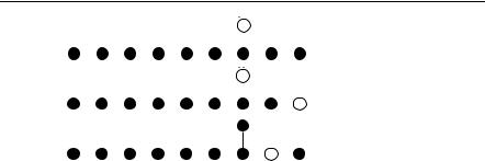
Unifying R-Symmetry in M-Theory

395

tion. Using the level decomposition one can further reduce this number by starting from a representation of the subalgebra (which obviously constitutes a necessary condition). Then the sufﬁcient consistency conditions involve only levels = 0 and= 1 (basically since there are only single lines in the E10 Dynkin diagram). For the so(10) subalgebra of K(e10) the recipe for constructing K(e10) representations is:

1.Start from an so(10) representation which we call the tentative K(e10) representation. This deﬁnes the action of the J ab generators within K(e10) on the tentative representation.

2.Make a general ansatz for the action of J abc on the tentative representation from so(10) representation theory.

3.Verify that the second line of (11) holds for the case when some of indices are

identical on the tentative representation. When some indices are identical the term with six anti-symmetric indices drops out.3 If there is a solution for the general ansatz then the tentative representation gives rise to a full consistent representation of K(e10).

For the other subalgebras the procedures are similar. Since it involves the tensors arising in the corresponding level decompositions we do not detail them here in order to keep the exposition simple.

We now construct the gravitino (vector-spinor) representation of K(e10) following the steps above. The vector-spinor of so(10) is reducible of dimension 320 and consists of the irreducible pieces 288 32 corresponding to the Γ -traceless part and the Γ -trace. We denote the vector-spinor by ψa and suppress the spinor index. The so(10) generators J ab act on ψa by4

J ab ψc	=	1	Γ ab ψc	+	2δ[a ψ b].	(12)

		2
					c

In the general ansatz for the J abc action there are three terms and the solution to the necessary commutation condition (11) leads to [10, 13]

J abc ψd	=	1	Γ abc ψd	+	4δ[a	Γ b ψ c]	−	Γd [ab ψ c].	(13)
		2
					d

That there exists a solution to the consistency condition implies that there is a representation of K(e10) of dimension 320. One can check that this is in fact an irreducible representation since the Γ -trace no longer separates once J abc is considered. We have thus proved that K(e10) has an irreducible 320 representation. Under the so(10) subalgebra it decomposes according to

320	−→ 288 32
K(e10)	so(10)	(14)

3That this is sufﬁcient follows from the precise expressions for the simple K(e10) generators xi of (6) in terms of components of the J ab and J abc which can be found in [11].

4Here, Γ a are the real (32 × 32) SO(10) Γ -matrices and Γ ab = Γ [a Γ b] etc.

396	Axel Kleinschmidt

as required. We denote this representation by Ψ since it can be deﬁned independently of the so(10) subalgebra under which it is more conveniently written as ψa .

We now turn to the decompositions under the subalgebras relevant for type IIA and type IIB. They were derived in [26] and we reproduce the results here as5

320	−→ (128 16) (128 16) 16 16
K(e10)	soA(9)	(15)

for type IIA, where the last two 16s are the dilatini, and

320	−→ ((128, 2) (16, 2)) (16, 2)
K(e10)	soB (9) so(2)	(16)

for type IIB. Here, the last doublet of 16s corresponds to the IIB dilatini. Since we are only dealing with the spatial Lorentz group so(9) different chiralities are not properly distinguished. The calculation shows, however, that the two doublets of 16s arise differently and in the covariant calculation one can show that indeed all chiralities also fulﬁll the necessary requirements to answer the ﬁrst question raised in the introduction afﬁrmatively: The group K(E10) contains the subalgebras required by the M-theory picture and has a spinorial representation with the correct number of components which branches correctly to the fermionic ﬁelds of the maximal supergravity theories.

3 Dynamics

To further substantiate the signiﬁcance of K(E10) and its 320 representation Ψ for an algebraic approach to M-theory we now turn to studying a dynamical equation for Ψ and its relation to the fermionic dynamics in the various maximal supergravities.

Since time is treated separately in the E10 context and all dynamical equations in the bosonic sector are time evolution equations a natural ansatz for the fermionic equation is

Dt Ψ = 0.

(17)

This is a Dirac equation for the K(e10) vector-spinor coupled minimally to a K(e10) connection Qt via the covariant derivative

Dt = ∂t − Qt ,

(18)

where Qt K(e10) acts on Ψ in the 320 representation. The gauge ﬁeld Qt transforms under t -dependent local K(E10) gauge transformations. As an K(e10) ele-

5 In [26] the subalgebra so(9, 9) was chosen for type IIA (instead of slA(9)) since this more naturally includes the mass term of the massive extension of IIA. That the result given here is also correct follows immediately from soA(9) so(10) and the branching rules for these groups.

Unifying R-Symmetry in M-Theory

397

ment, Qt can be expanded over so(10) in the generators (10) via

Qt =	1	Qab(0)J ab +				1	Qabc(1) J abc +	1	Qa(21)...a6 J a1	...a6
Qt =	2	Qab(0)J ab +				3!	Qabc(1) J abc +	6!	Qa(21)...a6 J a1	...a6
			1		(3)
	+				Qa0\|a1...a8 J a0\|a1...a8 + · · · .					(19)
	+		9	!	Qa0\|a1...a8 J a0\|a1...a8 + · · · .					(19)
				!

Since the action of all the K(e10) generators can be computed from multiple commutators of (12) and (13) the Dirac equation (17) can be evaluated to arbitrary level. In [10] it was evaluated up to sl(10) level three which is the level to which the ﬁeld content (9) is understood [8]. The resulting expression contains the gauge ﬁeld components Q( ) (for = 0, . . . , 3) contracted with various Γ -matrices multiplying the so(10) decomposed vector-spinor Ψ = (ψa ). Explicitly, we ﬁnd


				1		Qab(0)Γ ab		ψc − Qca(0)ψ a				1					Qa(11)a2a3 Γ a1a2a3 ψc
Dt ψc = ∂t ψc −												−
				4											12
	2							1											1
−		Qca(1)1a2 Γ a1 ψ a2 +								Qa(11)a2a3 Γc a1a2								ψ a3 −			Qa(21)...a6 Γ a1...a6 ψc
	3								6											1440
	1		Qca(2)1...a5 Γ a1					1					Qa(21)...a6 Γc a1...a5 ψ a6
+								...a4 ψ a5 −															(20)
	72										180
	2			(3)								2						(3)
−					Qa0\|a1...a8			Γc a1...a8 ψ a0 −										Qc\|a1...a8 Γ a1				...a7 ψ a8
	3 · 8!													3 · 7!
−	4				Qb(3\|ba)			Γ a1...a7 ψc −				1				Qb(3\|ba)			1...a7 Γc a1			...a6 ψ a7	+ · · · .
	3 · 8!						1...a7					3 · 6!

This equation has to be compared with the dynamical equation for the gravitino in D = 11 supergravity. From the analysis of the bosonic sector it is to be expected that gauge-ﬁxing is required in order to establish a connection between the K(e10) equation (20) and the supergravity equation [24]. Indeed it turns out [10] that one has to ﬁx a supersymmetry gauge (ψ0 − Γ0Γ a ψa = 0) for the fermions, a pseudoGaussian gauge (Et a = 0) for the vielbein and a Coulomb gauge (A0ab = 0) for the gauge potential. In this case the supergravity equation (to lowest fermion order) takes almost the same form as (20) but where the gauge ﬁeld components take the values [10, 11]


Qab(0)(t ) = −N ω0 ab (t, x0),				1
		Qa(21)...a6 (t ) = −					N a1...a6b1...b4 Fb1...b4 (t, x0),
					4	!
(1)	(t ) = N F0abc (t, x0),	(3)	(t ) =	3			(21)

Qabc		Qa0\|a1...a8		2 N a1...a8b1b2 ωb1 b2a0 (t, x0).

Here, ω0 ab and ωa bc are ‘electric’ and ‘magnetic’ components of the spin connection in ﬂat indices; similarly F0abc and Fb1...b4 are electric and magnetic components of the four-form ﬁeld strength in ﬂat indices. The lapse N = Et 0 is needed to convert the objects on the right hand sides into components of a world-line tensor Qt .

398 Axel Kleinschmidt

The equations (21) are valid only at a ﬁxed spatial point x0 and in order to match (20) to the supergravity equation higher spatial gradients of the ﬁelds (and the lapse) have to be ignored. Furthermore, the spatial spin connection must have vanishing trace ωb ba = 0 at x0. More details can be found in [10, 11].

To summarise, with the use of the ‘dictionary’ (21) we have succeeded in turning a truncated version of the D = 11 gravitino equation of motion into a K(E10) covariant Dirac-equation of the type (17). Although not explicitly proved in the type IIB case, one can expect that the very same equation (17) also describes the correct fermionic dynamics of type IIA and IIB by using the decompositions of K(e10) detailed in (15) and (16).

Thus we arrive at the main result: K(E10) is not only a viable candidate for a kinematical uniﬁcation of the fermionic symmetries of all maximal supergravity theories but also can partially be established as a symmetry of the dynamical equations for the fermions.

4 Discussion

4.1 Remarks

Here, we only brieﬂy sketch some related points and comment on a fully covariant reformulation of the above results.

There exists also a 32 representation of K(e10) which was called ‘Dirac-spinor’ in [12, 10]. This representation is relevant for the supersymmetry parameter and similarly has the correct branching to the various maximal supergravity theories’ Lorentz and R-symmetries [26].

Both the 320 and the 32 representations of K(e10) are unfaithful since they are ﬁnite-dimensional representations of an inﬁnite-dimensional algebra. This implies that K(e10) is not a simple Lie algebra but has non-trivial quotients. These one arrives at by factoring out the ideals associated with the unfaithful representations [11]. In the case of the 32 Dirac-spinor the quotient is so(32) which has been conjectured as a generalised holonomy in [14, 18]. Since K(E10) acts not only on the Dirac-spinor but also on the 320 gravitino (which SO(32) does not) it is more general than these conjectured holonomies. Furthermore, certain global issues [22] are resolved in K(E10) [10].

As mentioned in the introduction, the M-theoretic properties of K(E10) were derived following similar results in the bosonic sector [35, 33, 34, 8, 23, 25]. The bosonic ﬁelds are realised via a coset construction E10/K(E10) where K(E10) also acts as a local gauge symmetry. It is non-trivial, but true, that the relation between the gauge connection appearing in the bosonic analysis and the one in the fermionic analysis are related in precisely the same way to the supergravity quantities via (21).

It can also be shown that K(E11) (if equipped with the temporal involution of [16]) allows for a fermionic representation of dimension 352 = 320 + 32 if written

Unifying R-Symmetry in M-Theory

399

over SO(1, 10) [26]. The IIA and IIB decompositions of this fully covariant gravitino give the correct achiral and chiral fermionic spectra in a covariant fashion so that all the results of Sect. 2 carry over to K(E11). However, it is not clear how to write a K(E11) covariant and space-time covariant dynamical equation for this gravitino which generalises the Dirac equation (17). An obvious candidate is

D/ Ψ = 0,

(22)

where D/ = Γ M DM = Γ M (∂M − QM ). There are a number of subtleties with this suggestive notation that need to be clariﬁed. Firstly, DM should be K(E11) covariant meaning that the gauge ﬁelds transform correctly under K(E11). By augmenting an E11/K(E11) coset construction by a Borisov–Ogievetsky type construction as in [35] this can probably be achieved. The second problematic point is the symbol Γ M used above since Γ M is not an K(E11) invariant tensor and so spoils the K(E11) covariance of the equation even if DM transforms correctly. In line with the philosophy of [36] one should probably replace eleven-dimensional space-time indices M by indices taking values in an inﬁnite-dimensional highest weight representation of E11 generalising the translation vector to an E11 object. It remains to be seen whether one can make sense of (22) in this framework.

4.2 Outlook

From the discussion in the introduction it is clear that in order to complete the M- theory picture a number of things need to be included in the present algebraic framework, the most pressing of which we brieﬂy discuss now.

Firstly, M-theory should also include the non-maximal heterotic E8 × E8 and SO(32) string theories as well as the SO(32) type I superstring. At low energies this requires ﬁtting the heterotic D = 10 supergravity with gauge groups SO(32) and E8 × E8 into the E10 σ -model or some more general model. As a ﬁrst step it was shown in [23, 17] that the pure type I supergravity (without any vector multiplets) can be interpreted as a subsector of the E10 model. It would be gratifying to see a relation between the algebraic approach taken here and the issue of anomaly freedom.

Secondly, M-theory presumably is a theory of strings and other extended objects. The analysis so far only covered point particles since properties of the low energy ﬁeld theories were studied. It is not clear if the symmetries found need to be modiﬁed when extended objects are also considered. Results from U-duality [19, 32] suggest that the continuous symmetry gets broken to some discrete arithmetic group and ﬁrst ideas in this direction were discussed in [4]. A different route was taken in [7, 9] where string induced higher derivative corrections to the low energy effective action were studied in relation to E10 and good agreement between the algebraic structure and conjectured properties of these correction terms was found (see also [29]).

400	Axel Kleinschmidt

Thirdly, the bosonic ﬁelds appear through the inﬁnite—dimensional coset space E10/K(E10) whereas the fermionic ﬁelds presently are conﬁned to a ﬁnite—dimen- sional, unfaithful representation of K(E10). This seems problematic from a supersymmetry point of view. This dichotomy is partly related to the difference in order of the equations of motion for bosons and fermions. The fermionic ﬁeld equations are ﬁrst order whereas the bosonic ones are second order (allowing for dualisations and triggering for example the inﬁnite duality cascade in D = 2). It would be nice to overcome this obstacle through the construction of an appropriate faithful fermionic representation of K(E10).

Finally, on the purely mathematical side it could be hoped that a proper understanding of the relation between E10 and M-theory may lead to a new presentation of the E10 structure itself. Since its inception in the late 1960s [20, 30] the theory of indeﬁnite Kac–Moody algebras has produced few results which truly penetrate the structure of these fascinating objects.

Acknowledgements The author is grateful to Thibault Damour and Hermann Nicolai for very stimulating collaborations leading to the results presented here and would like to thank the organisers of the ICMP 2006 conference for providing an interesting congress. This work was partially supported by the European Research and Training Networks ‘Superstrings’ (contract number MRTN-CT-2004-512194) and ‘Forces Universe’ (contract number MRTN-CT-2004-005104).

References

1.E.A. Bergshoeff, M. de Roo, S.F. Kerstan, and F. Riccioni, IIB supergravity revisited. J. High Energy Phys. 0508, 098 (2005). hep-th/0506013

2.E.A. Bergshoeff, M. de Roo, S.F. Kerstan, T. Ortin, and F. Riccioni, IIA ten-forms and the gauge algebras of maximal supergravity theories. hep-th/0602280

3.S. Berman, On generators and relations for certain involutory subalgebras of Kac-Moody Lie algebra. Commun. Algebra 17, 3165–3185 (1989)

4.J. Brown, O.J. Ganor, and C. Helfgott, M theory and E10: Billiards, branes and imaginary roots. hep-th/0401053

5.E. Cremmer and B. Julia, The SO(8) supergravity. Nucl. Phys. B 159, 141 (1979)

6.E. Cremmer, B. Julia, H. Lu, and C.N. Pope, Dualisation of Dualities, I. Nucl. Phys. B 523, 73–144 (1998). hep-th/9710119

7.T. Damour and H. Nicolai, Higher order M theory corrections and the Kac-Moody algebra E10. Class. Quantum Gravity 22, 2849 (2005). hep-th/0504153

8.T. Damour, M. Henneaux, and H. Nicolai, E10 and a “small tension expansion” of M-theory. Phys. Rev. Lett. 89, 221601 (2002). hep-th/0207267

9.T. Damour, A. Hanany, M. Henneaux, A. Kleinschmidt, and H. Nicolai, Curvature corrections and Kac-Moody compatibility conditions. Gen. Relativ. Gravit. 38, 1507 (2006). hep-th/0604143

10.T. Damour, A. Kleinschmidt, and H. Nicolai, Hidden symmetries and the fermionic sector of eleven-dimensional supergravity. Phys. Lett. B 634, 319 (2006). hep-th/0512163

11.T. Damour, A. Kleinschmidt, and H. Nicolai, K(E10), supergravity and fermions. J. High Energy Phys. 0608, 046 (2006). hep-th/0606105

12.S. de Buyl, M. Henneaux, and L. Paulot, Hidden symmetries and Dirac fermions. Class. Quantum Gravity 22, 3595 (2005). hep-th/0506009

Unifying R-Symmetry in M-Theory

401

13.S. de Buyl, M. Henneaux, and L. Paulot, Extended E8 invariance of 11-dimensional supergravity. J. High Energy Phys. 0602, 056 (2006). hep-th/0512292

14.M. Duff and J.T. Liu, Hidden space-time symmetries and generalized holonomy in M theory. Nucl. Phys. B 674, 217–230 (2003). hep-th/0303140

15.F. Englert and L. Houart, G +++ invariant formulation of gravity and M-theories: Exact intersecting brane solutions. J. High Energy Phys. 0405, 059 (2004). hep-th/0405082

16.F. Englert and L. Houart, G +++ invariant formulation of gravity and M-theories: Exact BPS solutions. J. High Energy Phys. 0401, 002 (2004). hep-th/0311255

17.C. Hillmann and A. Kleinschmidt, Pure type I supergravity and DE10. Gen. Relativ. Gravit. 38, 1861 (2006). hep-th/0608092

18.C. Hull, Holonomy and symmetry in M theory. hep-th/0305039

19.C.M. Hull and P.K. Townsend, Unity of superstring dualities. Nucl. Phys. B 438, 109–137 (1995). hep-th/9410167

20.V.G. Kac, Simple graded Lie algebras of ﬁnite growth. Funkt. Anal. ego Prilozh. 1, 82–83 (1967); English translation: Funct. Anal. Appl. 1, 328–329 (1967)

21.V.G. Kac, Inﬁnite Dimensional Lie Algebras, 3rd edn. Cambridge University Press, Cambridge (1990)

22.A. Keurentjes, The topology of U Duality (sub)groups. Class. Quantum Gravity 21, 1695– 1708 (2004). hep-th/0309106

23.A. Kleinschmidt and H. Nicolai, E10 and SO(99) invariant supergravity. J. High Energy Phys. 0407, 041 (2004). hep-th/0407101

24.A. Kleinschmidt and H. Nicolai, Gradient representations and afﬁne structures in AEn. Class. Quantum Gravity 22, 4457–4488 (2005). hep-th/0506238

25.A. Kleinschmidt and H. Nicolai, IIB supergravity and E10. Phys. Lett. B 606, 391 (2005). hep-th/0411225

26.A. Kleinschmidt and H. Nicolai, IIA and IIB spinors from K(E10). Phys. Lett. 637, 107–112 (2006). hep-th/0603205

27.A. Kleinschmidt and H. Nicolai, K(E9) from K(E10). hep-th/0611314

28.A. Kleinschmidt, I. Schnakenburg, and P. West, Very extended Kac–Moody algebras and their interpretation at low levels. Class. Quantum Gravity 21, 2493–2525 (2004). hep-th/0309198

29.N. Lambert and P. West, Enhanced coset symmetries and higher derivative corrections. Phys. Rev. D 74, 065002 (2006). hep-th/0603255

30.R.V. Moody, Lie algebras associated with generalized Cartan matrices. Bull. Am. Math. Soc. 73, 217–221 (1967)

31.H. Nicolai and T. Fischbacher, Low level representations of E10 and E11. Contribution to the Proceedings of the Ramanujan International Symposium on Kac–Moody Algebras and Applications, ISKMAA-2002, Chennai, India, 28–31 January. hep-th/0301017

32.N.A. Obers and B. Pioline, M Theory and U Duality. Phys. Rep. 318, 113–225 (1999). hep-th/9809039

33.I. Schnakenburg and P.C. West, Kac–Moody symmetries of 2B supergravity. Phys. Lett. B 517, 421–428 (2001). hep-th/0107081

34.I. Schnakenburg and P.C. West, Massive IIA supergravity as a nonlinear realization. Phys. Lett. B 540, 137–145 (2002). hep-th/0204207

35.P.C. West, E11 and M theory. Class. Quantum Gravity 18, 4443–4460 (2001). hep-th/0104081

36.P. West, E11, SL(32) and central charges. Phys. Lett. B 575, 333–342 (2003). hep-th/0307098

37.P. West, Very extended E8 and A8 at low levels, gravity and supergravity. Class. Quantum Gravity 20, 2393–2406 (2003). hep-th/0212291

38.E. Witten, String theory dynamics in various dimensions. Nucl. Phys. B 443, 85–126 (1995) hep-th/9503124

<<< < Предыдущая 23 24 25 26 27 28 29 30 31 32 33 3435 / 6835 36 37 38 39 40 41 42 43 44 45 46 47 > Следующая >>>

Соседние файлы в папке Diss

#
27.03.20161.6 Mб5127.pdf
#
27.03.20167.05 Mб17228.pdf
#
27.03.20161.31 Mб523.pdf
#
27.03.2016838.41 Кб484.pdf
#
27.03.2016451.11 Кб425.pdf
#
27.03.201615.34 Mб486 - 753p.pdf
#
27.03.2016451.11 Кб406.pdf
#
27.03.2016499.39 Кб457.pdf
#
27.03.20161.47 Mб438.pdf
#
27.03.201615.42 Кб41Введение.docx
#
27.03.201619.78 Кб43Список литературы.docx

	V = {0, 1}d ,
	E = {(v, v ) V × V : \|x − x \| = 1)},
where \|v − v \| =	d
where \|v − v \| =	i=1 \|v(i) − v (i)\| is the Hamming distance in V .