Добавил:

Upload Опубликованный материал нарушает ваши авторские права? Сообщите нам.

Вуз:

Национальный исследовательский университет «МИЭТ»

Предмет:

[НЕСОРТИРОВАННОЕ]

Файл:

Diss / 6 - 753p.pdf

Скачиваний:

Добавлен:

27.03.2016

Размер:

15.34 Mб

Скачать

☆

<<< < Предыдущая 34 35 36 37 38 39 40 41 42 43 44 4546 / 6846 47 48 49 50 51 52 53 54 55 56 57 58 > Следующая >>>

ABCD and ODEs

689

K/Baa ; the model-dependent integer K corresponds to the degree of fusion (see for example [16]).

3 The Pseudo-Differential Equations

To describe the pseudo-differential equations corresponding to the An−1, Bn, Cn and Dn simple Lie algebras we ﬁrst introduce some notation. We need an nth-order differential operator [9]

Dn(g) = D(gn−1 − (n−1)) D(gn−2 − (n−2)) . . . D(g1 − 1) D(g0), (19)

D(g) =	d	−	g	,	(20)

	dx		x

depending on n parameters

g = {gn−1, . . . , g1, g0}, g† = {n − 1− g0, n − 1− g1, . . . , n − 1− gn−1}. (21)

Also, we introduce an inverse differential operator (d/dx)−1, generally deﬁned through its formal action

	d	1		xs	1
		−	xs =		+	,	(22)
	dx	−	xs =	s	1	,	(22)
			+
and we replace the simple ‘potential’ P (E, x) = (x2M − E) of (5) with
PK (E, x) = (xh M/K − E)K .							(23)

Using the notation of Appendix B in [12] the proposed pseudo-differential equations are reported below.

An−1 models

The An−1 ordinary differential equations are

Dn(g†)χn†−1(x, E) = PK (x, E)χn†−1(x, E),

(24)

with the constraint

n−1 g

i =

n(n−1)

and the ordering g

< g

< n

−

i < j .

i=0

γ (g)

We introduce the

alternative set of parameters γ

(g)

= {

}

a−1

a(h

−

γa =

gi −

(25)

h M

i=0

690 Patrick Dorey, Clare Dunning, Davide Masoero, Junji Suzuki and Roberto Tateo

The solution χn†−1(x, E) is speciﬁed by its x 0 behaviour
χn†	1 xn−1−g0 + subdominant terms, (x → 0+).	(26)
−

In general, this function grows exponentially as x tends to inﬁnity on the positive real axis. In Appendix B of [12], it was shown that the coefﬁcient in front of the leading term, but for an irrelevant overall constant, is precisely the function Q(1)(E, γ ) appearing in the Bethe Ansatz, that is

†		M xM+1
χn−1	Q(1)(E, γ (g)) x(1−n) 2 e M+1 + subdominant terms, (x → ∞).
Therefore, the set of Bethe ansatz roots
		{Ei(1)} ↔ Q(1)(Ei(1), γ ) = 0
coincide with the discrete set of E values in (24) such that
	†	M xM+1
	χn−1	o x(1−n) 2 e M+1 , (x → ∞).

This condition is equivalent to the requirement of absolute integrability of

x(n−1)	M	xM+1	†
x(n−1)	2 e−	M+1	χn−1	(x, E)

(27)

(28)

(29)

(30)

on the interval [0, ∞). It is important to stress that the boundary problem deﬁned above for the function χn†−1 (26) is in general different from the one discussed in Sects. 3 and 4 in [12] involving ψ (x, E). The latter function is instead a solution to the adjoint equation of (24) and characterised by recessive behaviour at inﬁnity. Surprisingly, the two problems are spectrally equivalent and lead to identical sets of Bethe ansatz roots.

Dn models

The Dn pseudo-differential equations are

Dn(g†)	dx −		1
Dn(g†)	dx −		Dn(g)χ2n−1(x, E)
		d

= PK (x, E)	d	PK (x, E) χ2n−1(x, E).	(31)
	dx

Fixing the ordering gi < gj < h /2, the g ↔ γ relationship is

ABCD and ODEs

691

γa

a−1 gi

−

h ,

1, . . . , n

−

(32)

= h M

i=0

γn

n−1 gi

h ,

−

= h M

− 2

i=0

(33)

γn

n−2 gi

gn 1

n − 2

h .

= h M

−

i=0

The solution is speciﬁed by requiring

χ2n−1 xh −g0 + subdominant terms,

(x → 0+),

(34)

M xM+1

(x → ∞).

χ2n−1 Q(1)(E, γ (g)) x−h 2 e M+1 + subdominant terms,

(35)

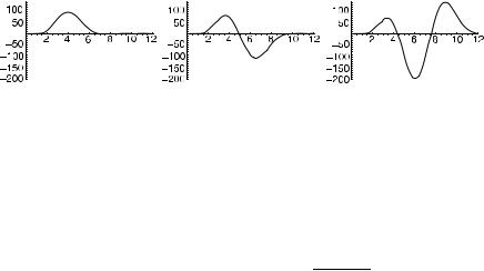
Figure 1 illustrates Ψ (x, E)

xM+1

−

(x, E) for the ﬁrst three eigen-

2 e− M+1 χ2n 1

values of the D4

pseudo-differential equation deﬁned by K=1, M = 1/3 and

g = (2.95, 2.3, 1.1, 0.2).

Fig. 1 Lowest three functions Ψ (x, E) for a D4 pseudo-differential equation

Bn models

The Bn ODEs are

PK (x, E)χ2†n

Dn(g†)Dn(g)χ2†n

1(x, E)

PK (x, E)

1(x, E). (36)

−

With the ordering gi

< gj < h /2, the g ↔ γ relation is

a−1

γa

−

h .

(37)

i=0

The asymptotic behaviours about x = 0 and x = ∞ are respectively

692	Patrick Dorey, Clare Dunning, Davide Masoero, Junji Suzuki and Roberto Tateo
	χ2†n−1 xh −g0 + subdominant terms, (x → 0+) ,						(38)
and
2n−1		M	xM+1	+		→ ∞
χ †	Q(1)(E, γ (g)) x	−h 2	e M+1		subdominant terms, (x	).	(39)

Cn models

The pseudo-differential equations associated to the Cn systems are

Dn(g†)	dx		Dn(g) χ2n+1	(x, E) = PK (x, E) dx −		1
						PK (x, E) χ2n+1(x, E)
		d			d

(40) with the ordering gi < gj < n. The relation between the g’s and the twist parameters in the BAE is

γa

a−1 gi

an ,

γn

n−1 gi

(41)

= h M

−

= h M

−

i=0

and

χ2†n 1 x2n−g0 + subdominant terms,

(x → 0+),

(42)

xM+1

†

+ subdominant terms,

(x → ∞).

(43)

χ2n+1

Q(1)(E, γ )x−nM e M+1

Using a generalisation of Cheng’s algorithm, the zeros of Q(1)(E, γ ) can be found numerically and shown to match the appropriate Bethe ansatz roots [12].

In general, the ‘spectrum’ of a pseudo-differential equation may be either real or complex. In the An−1, Bn, Dn models with K = 1,1 the special choice gi = i leads to pseudo-differential equations with real spectra, a property which is expected to hold for a range of the parameters g (see, for example, [9]). The K > 1 generalisation of the potential (23), proposed initially by Lukyanov for the A1 models [17] but expected to work for all models, introduces a new feature. The eigenvalues corresponding to a K = 2, 3 and K = 4 case of the SU(2) ODE are illustrated in Fig. 2.

The interesting feature appears if we instead plot the logarithm of the eigenvalues as in Fig. 3. We see that the logarithm of the eigenvalues form ‘strings’, a wellknown feature of integrable models. The string solutions approximately lie along lines in the complex plane, the deviations away from which can be calculated [12] using either WKB techniques, or by studying the asymptotics of the Bethe ansatz equations directly.

1 The Cn spectrum is complex for any integer K ≥ 1.

<<< < Предыдущая 34 35 36 37 38 39 40 41 42 43 44 4546 / 6846 47 48 49 50 51 52 53 54 55 56 57 58 > Следующая >>>

Соседние файлы в папке Diss

#
27.03.20161.6 Mб6727.pdf
#
27.03.20167.05 Mб20428.pdf
#
27.03.20161.31 Mб673.pdf
#
27.03.2016838.41 Кб634.pdf
#
27.03.2016451.11 Кб575.pdf
#
27.03.201615.34 Mб646 - 753p.pdf
#
27.03.2016451.11 Кб556.pdf
#
27.03.2016499.39 Кб607.pdf
#
27.03.20161.47 Mб598.pdf
#
27.03.201615.42 Кб56Введение.docx
#
27.03.201619.78 Кб58Список литературы.docx