


Energy Diffusion |
545 |
Rigorous results can be proven for the harmonic case with γ > 0 [2, 3]. It turns out that κ is finite if system is pinned or in dimension d ≥ 3, while the 1 and 2 dimensional unpinned cases are superdiffusive.
4 Kinetic Limits: Phonon Boltzmann Equation
The harmonic case is enough simple to obtain some non-equilibrium results. In [5] we consider the hyperbolic scaling in a weak noise limit. Noise is rescaled by multiplying its strength γ by . This way the effect of the noise per particle remains finite in the macroscopic scale (that motivates the term kinetic in defining this limit). This is in the same spirit as the model of hard sphere with random collision considered in [15]. The right quantity to look here is the Wigner distribution of the energy, formally defined as
|
1 |
1/2 |
|
|
|
W (y, k, t ) = |
|
−1/2 ei2πyη/ ψ (k − η/2, t / ) ψ (k + η/2, t / ) dη (24) |
|||
2 |
|||||
where |
|
1 |
|
||
|
|
(ω(k)qˆ (k, t ) + ip(k,ˆ t )) |
|||
|
|
ψ (k, t ) = |
√ |
|
|
|
|
2 |
|||
here qˆ (k, t ), p(k,ˆ t ) are the Fourier transform of the qy (t ), py (t ), and ω(k) is the dispersion relation of the lattice, which in this one-dimensional nearest neighbour
case is |
given by ω(k) = c| sin(π k)| (acoustic dispersion). The result in [5] states |
|||
that W |
(y, k, t ) converges, as a distribution on R × [0, 1], to the solution of the |
|||
linear transport equation |
|
|
|
|
|
∂t W (y, k, t ) + |
ω (k) |
∂y W (y, k, t ) |
|
|
2π |
|
||
|
= γ C(k, k )(W (y, k , t ) − W (y, k, t ))dk. |
(25) |
||
In the deterministic case (γ = 0) this result was obtained by Dobrushin et al. in [9], see also [13]. The collision kernel C(k, k ) is positive and symmetric. It is computable explicitly (cf. [5]), but the important point is that C(k, k ) k2 for small k. This is a consequence of the conservation of momentum: long waves scatter very rarely. Because C(k, k ) is positive, (25) has a simple probabilistic interpretation: W is the density at time t of the energy of particles (phonons) of mode k. A phonon of mode k moves with velocity ω (k) and after an exponentially distributed random time of intensity γ C(k, k ) changes its mode to k . Defining a Markov jump
|
) in |
0, 1 |
] |
with jumping rate γ C, the position of the phonons is given |
|
process K(t t |
[ |
|
|
||
by Y (t ) = |
0 |
ω (K(s))ds. |
|||
Thermal conductivity can be computed from (25) (cf. [5]) and the results are in accord with the direct calculations done in [3].
546 |
Stefano Olla |
5 Levy’s Superdiffusion of Energy
As we mention in the previous section, phonons of small k scatter rarely, but their velocity ω (k), in the unpinned case, are still of order 1 as k → 0. This induces a superdiffusive behavior of these phonons. In [11], as application of new limit theorems for functionals of Markov chains and processes, we prove that, for α = 3/2,
Y ( −α t ) −→ L(t ) (26)
law
where L(t ) is a Levy α-stable process, i.e. a stochastic process with independent stationary increments and with L(1) distributed by a α-stable law. In terms of the solution W (y, k, t ) of (25) this result implies the convergence
lim |
| |
W ( −α t, −1y, k) |
u(t, y) |
2dk |
= |
0 |
(27) |
||
|
→ |
0 |
|
− ¯ |
| |
|
|
||
|
|
|
|
|
|
|
|
|
|
where u(t¯ , y) is the solution of the fractional heat equation |
|
|
|
||||||
|
|
|
|
∂t u¯ = −c(− |
y )α/2u¯. |
|
|
|
(28) |
where c is a positive constant.
In the pinned case all the above results are still valid, but since the velocity of the phonons ω (k) k for small k, we have a regular diffusive behavior, and α = 2.
It would be very interesting to understand how these results extends to the anharmonic cases. Equation (25) will be substituted by the non-linear phonon Boltzmann equation [17]. In the unpinned one-dimensional case this equation still will produce a superdiffusion. Is it again of Levy type, or will have some non-Markovian terms?
References
1.G. Basile, PhD thesis, Université Paris Dauphine (2007)
2.G. Basile, C. Bernardin, and S. Olla, Momentum conserving model with anomalous thermal conductivity in low dimensional systems. Phys. Rev. Lett. 96(20), 4 (2006)
3.G. Basile, C. Bernardin, and S. Olla, Thermal conductivity for a momentum conserving model.
Commun. Math. Phys. 287(1), 67–98 (2009)
4.G. Basile, L. Delfini, S. Lepri, R. Livi, S. Olla, and A. Politi, Anomalous transport and relaxation in classical one-dimensional models. Eur. J. Phys. Spec. Top. 151(1), 85–93 (2007)
5.G. Basile, S. Olla, and H. Spohn, Wigner functions and stochastically perturbed lattice dynamics. Arch. Ration. Mech. Anal. (2009). doi:10.1007/s00205-008-0205-6
6.C. Bernardin and S. Olla, Non-equilibrium macroscopic dynamics of a chain of anharmonic oscillators (in preparation)
7.F. Bonetto, J. Lebowitz, J. Lukkarinen, and S. Olla, Heat conduction and entropy production in anharmonic crystals with self-consistent stochastic reservoirs. J. Stat. Phys. 134(5–6), 1097– 1119 (2009). doi:10.1007/s10955-008-9657-1
8.F. Bonetto, J. Lebowitz, and L. Rey-Bellet, Fourier’s law: A challenge to theorists. In: Fokas, A., Grigoryan, A., Kibble, T., Zegarlinski, B. (eds.), Mathematical Physics 2000. Imperial College, London (2000)
Energy Diffusion |
547 |
9.R.L. Dobrushin, A. Pellegrinotti, Yu.M. Suhov, and L. Triolo, One-dimensional harmonic lattice caricature of hydrodynamics. J. Stat. Phys. 43(3–4), 571–607 (1986)
10.T. Funaki and H. Spohn, Motion by mean curvature from the Ginzburg-Landau interface model. Commun. Math. Phys. 185, 1–36 (1997)
11.M. Jara, T. Komorowski, and S. Olla, Limit theorems for additive functionals of a Markov chain. Ann. Appl. Probab. (2009)
12.S. Lepri, R. Livi, and A. Politi, Heat conduction in chains of nonlinear oscillators. Phys. Rev. Lett. 78, 1896 (1997)
13.A. Mielke, Macroscopic behavior of microscopic oscillations in harmonic lattices via WignerHusimi transforms. Arch. Rat. Mech. Anal. 181, 401–448 (2006)
14.S. Olla, S.R.S. Varadhan, and H.-T. Yau, Hydrodynamical limit for a Hamiltonian system with weak noise. Commun. Math. Phys. 155(3), 523–560 (1993)
15.F. Rezakhanlou, Boltzmann-Grad limits for stochastic hard sphere models. Commun. Math. Phys. 248(3), 553–637 (2004)
16.Z. Rieder, J.L. Lebowitz, and E. Lieb, Properties of a harmonic crystal in a stationary nonequilibrium state. J. Math. Phys. 8, 1073 (1967)
17.H. Spohn, The phonon Boltzmann equation, properties and link to weakly anharmonic lattice dynamics. J. Stat. Phys. 124(2–4), 1041–1104 (2006)

550 |
Enrique R. Pujals |
Following this approach, for a long time it has been a goal in the theory of dynamical systems to describe the dynamics from the generic viewpoint, that is, describing the dynamics of “big sets” (residual, dense, etc.) of the space of all dynamical systems. In other words: can we describe the behavior in the long run of typical trajectories for the ‘majority’ of systems?
In this sense, to study a dynamic system is to look for mathematically describable patterns that a system tends to settle. These sets are sets which are “dynamically indecomposable”, “invariant”, and “isolated” (also called elementary pieces) that contain the recurrent part of the dynamic (the so called nonwandering set). Invariant, means that any trajectory starting in the set remains in the set; dynamically indecomposable means that the set is transitive (i.e., contains trajectories which are dense in the set); isolated, means that the set is maximal invariant (i.e., the set is given by the trajectories that for the past and the future remains in a neighborhood of the set).
During the early times of nonconservative dynamics was a common sense that “non pathological” systems behaves in a very simple form: the nonwandering set consisting of finitely many periodic elements. The achievement of Peixoto that an open and dense subset of C1 vector fields on surfaces consist of the now-called Morse-Smale systems is paradigmatic of this view. However, in the early sixties (by Anosov and Smale and following Birkhoff, Cartwright and Littlewood, etc.) it was shown that “chaotic behavior” may exist within stable systems and this was the starting point of the hyperbolic theory and the modern nonconservative dynamical systems theory. A major result in this theory is the fact that for these systems (nowadays called hyperbolics, see Sect. 2.1), the nonwandering set can be decomposed into finitely many compact, disjoint and transitive pieces. Although this pieces could exhibit a chaotic behavior there are just finitely many of them and this recover the old vision by replacing finitely many periodic elements by these finitely many “non-trivial elementary” pieces.
It was soon realized that hyperbolic systems were not as universal as was initially thought: there were given examples of open sets of diffeomorphism were none of them are hyperbolic. Nevertheless in all these new examples the nonwandering set still decompose into finitely many compact, disjoint and transitive pieces. Moreover, this phenomena holds in a robust way: Any perturbation of the initial system still has a only a finite number of transitive pieces.
It was through the seminal work of Newhouse (see [41–43]) where a new phenomena was shown: the existence of infinitely many periodic attractors (today called Newhouse’s phenomena) for residual subsets in the space of Cr diffeomorphisms
(r 2) of compact surfaces. The underlying mechanism here was the presence of a homoclinic bifurcation named homoclinic tangency: non-transversal intersection of the stable and unstable manifold of a periodic point (see Sect. 3).
In the light of those results, the following dichotomy was formulated for generic dynamics (see [1] for more details):
1.Robust/Tame dynamics: those having in a robust way, finitely many elementary dynamical pieces in the ambient manifold;
Trying to Characterize Robust and Generic Dynamics |
551 |
2.Wild dynamics (Newhouse’s phenomena): those with infinitely many elementary pieces having independent dynamical behaviors.
Once the dichotomy is presented, one tried to understand the structure related to the presence of robust phenomena and the universal mechanisms that lead to lack of robustness and to wild dynamics. Following this approach, the theory moves in the ongoing directions:
1.Characterization of the properties and structure that robust (tame) dynamics have; in particular, the study and characterization of isolated transitive sets that remain transitive for all nearby systems (robust transitivity).
2.Characterization of the properties and structure that wild dynamics exhibit.
3.Characterization of universal mechanisms (understood as homoclinic bifurcations) that lead to robust and wild dynamics.
These problems are all related to each other and in many cases provide a conceptual framework that makes possible to understand a twofold problem: the relation between mechanisms and phenomenas. As we are going to show, a global panorama, although partial and very incomplete, is beginning to appear. In this approach, local mechanism are used to characterize global properties of the dynamics. In this sense, the strategy consists in building new mechanisms, enough for characterizing all the possible behaviors. Therefore, one focus is to understand which are the mechanisms that make a transitive either to be robust or to “explode/implode” in infinitely many other sets.
In the present note we focus our attention on diffeomorphism acting on a smooth boundaryless compact manifold. Some references to the flow case are also made. Moreover, the present note focus on nonconservative systems; however, we mention some results for the conservative case (recall that in this case, a long and successful theory had been developed where the KAM theorem is the major highlight).
In Sect. 2 we extend ourselves explaining the relevant examples of robust dynamics. In the three following subsections we details the main structure that those systems exhibit. In Sect. 3 we focus in the main mechanisms that generate wild dynamics and in Sect. 4 we expose partial results in the direction to describe generic type of dynamics.
2Robust Transitivity: Hyperbolicity, Partial Hyperbolicity and Dominated Splitting
A diffeomorphisms f : M → M is robustly transitive if every diffeomorphism in a C1 neighborhood has dense orbits. More generally:
An invariant compact set Λ is robustly transitive if there is an open neighborhood U of Λ and a neighborhood V of the diffeomorphism f in Diff1(M) such that for every g V the maximal invariant set Λg = n Z gn(U ) of g in U is a transitive set.
552 |
Enrique R. Pujals |
The description of these systems is an important challenge: on the one hand, being robust, they can not be ignored in any global picture of dynamical systems; on the other hand, their dynamics is often chaotic.
The typical models showing robust properties are the well known Anosov maps (as examples of global hyperbolic dynamics) and the Smale’s horseshoes (as examples of local hyperbolic ones).
However, it was shown that there are open sets in the space of dynamics which are nonhyperbolic although transitive. Indeed, in [52], an open set of non-hyperbolic transitive diffeomorphisms in the 4-torus were exhibited (open sets of diffeomorphisms exhibiting hyperbolic periodic points of different indices inside a transitive set). On one hand, these examples were a serious blow at the time, since they meant that even such seemingly simple situations, exhibiting a unique dynamical piece, cannot be understood within the framework of hyperbolicity. On the other hands these systems exhibit a weaker form of hyperbolicity called partial hyperbolicity: the tangent bundle is allowed to split into Df -invariant subbundles T M = Es Ec Eu, such that the behavior of vectors in Es , Eu is similar to the hyperbolic case, but vectors in Ec may be neutral for the action of the tangent map. See Sect. 2.2 for more details.
But the story about robust transitivity does no finish with the partially hyperbolic ones: In the late 90’s, examples of robust transitive dynamics without any hyperbolic subbundles were exhibited. More precisely, in [15] was shown that there are robustly transitive diffeomorphisms in the 4-torus which have no expanding or contracting invariant sub-bundle; therefore, they are neither hyperbolic nor partially hyperbolic. However, those examples still exhibit a some kind of structure of their tangent dynamics: there is a splitting T M = Ecs Ecu preserved by the derivative of the map, called dominated splitting, where Ecs and Ecu are indecomposable and nonhyperbolic. See Sect. 2.3 for more details.
All those examples pushes the theory in the following directions:
1.The general characterization of isolated transitive sets that remain transitive for all nearby systems;
2.The dynamical consequences of weaker forms of hyperbolicity;
3.The characterization of universal mechanisms that could lead to robustly nonhyperbolic behavior.
Respect to the first question proposed a general principle is concluded: robust dynamical phenomena reflect some robust structure of the tangent map.
In fact, in [35] for surface diffeomorphisms, in [25] for dimension three, and in [17] for any dimension it is shown that this is the main characteristic of C1-robust transitivity. More precisely, the following was proved:
Any C1-robust transitive diffeomorphism exhibits a dominated splitting such that its extremal bundles are uniformly volume contracted or expanded.
This last theorem has other formulations in terms of certain generic dichotomy and also in conservative terms: see [1, 10, 11, 13, 12, 5].
A similar theory can be developed for flows that include that includes the Geometric models for the Lorenz equations proposed in [2, 29]. Diverse results that
Trying to Characterize Robust and Generic Dynamics |
553 |
characterize robustly transitive flows with an equilibrium point have been developed. We refer to [38, 8, 4, 49] for further reading.
In the next subsection, we are going to extend ourselves in explaining the notion of hyperbolicity, partially hyperbolicity and dominated splitting. We also going to explain certain relevance that those models has in some physical problems: in the hyperbolic case we describe a mechanical model with hyperbolic dynamics; in the partial hyperbolic case, we explain certain construction in the context of symplectic dynamics which are relevant to the problem of Arnold’s diffusion; in the context of dominated splitting, we relate these dynamics with Gaussian thermostats and isokinetic dynamics.
2.1 Hyperbolicity
The study of hyperbolicity goes back to the work of Hadamard in 1898 concerning geodesic flows for surfaces with negative curvature, showing the density of closed geodesics and the instability of the flow with respect to initial conditions. In the 20s and 30s, Hedlund and Hopf showed that these flows are topologically mixing and that they are ergodic with respect to the Liouville measure.
Later, in [3] it was shown that geodesic flows for compact manifolds with negative sectional curvature are hyperbolic (Anosov) flows.
Let us start defining the notion of hyperbolicity for diffeomorphisms: Given a compact invariant set Λ M of a diffeomorphism f , one says that Λ is a hyperbolic set of f if the tangent bundle of Λ splits into two invariant sub-bundles: TΛM = Es Eu, and there are two constants λ < 0 and c > 0 such that the following properties hold:
1.Df n|Es < c exp(λn) for n > 0; that is, Es is uniformly contracted in the future.
2.Df −n|Eu < c exp(λn) for t > 0; that is, Eu is uniformly contracted in the past.
The classical example of hyperbolic diffeomorphisms are the Anosov ones where Λ is the whole manifold, and the Axiom A where in this case Λ is the nonwandering set and the periodic points are dense.
For a vector field X, a compact set Λ invariant by the flow is a hyperbolic set of Φt if the tangent bundle of Λ splits into three invariant sub-bundles: TΛM = Es [X] Eu, such that [X] is the subbundle induced by the vector field, and the subbundle Es is uniformly contracted in the future and Eu is uniformly contracted in the past. One of the most important property of hyperbolic systems is that in contrast to the instability of their orbits, the hyperbolic dynamics are stable in the sense that any perturbation of the system is conjugate to the initial one, meaning that the relevant dynamical behavior is actually the same, in some appropriate sense, again for all nearby systems. In particular, this shows that transitive hyperbolic systems (hyperbolic systems that have a dense trajectory) are in fact Cr robust transitive ones; i.e: any Cr small perturbation of the initial system remains transitive.
554 |
Enrique R. Pujals |
A long standing question has been whether there is a physical example of a Hamiltonian system with Anosov energy levels—i.e., the Hamiltonian flow is Anosov on some energy level sets. A positive answer to this question was given in the remarkable paper of [31] where the dynamics of a triple linkage is studied: three disks in a plane, free to rotate about pivots fixed in a triangle, but constrained by three rods connecting one point of each disk to a pivot x. For its free frictionless motion Hunt and Mackay proved existence of an open set of three linkage configurations for which the dynamics in each positive energy level set is a geodesic Anosov flow arising from negative curvature.
2.2 Partial Hyperbolicity
Given a closed invariant set Λ we say that it is strong partially hyperbolic if TΛM = Ess Ec Euu and there are constants 0 < σ −1 < γ −1 < 1 < γ < σ such that
|
Df |
|
|
< σ −1 |
< σ < |
|
Df |
1 |
|
−1 |
|
|
x |
|
Λ |
|
|
|
|
|
|
|
|
|
ss |
|
|
−uu |
|
|
|
|
|
|
|
|
|
|
|||||||||
|
|Ex |
|
1 |
|
|
|E |
|
|
|
1 |
|
|
|
|
|
|
|||||||
|
Df |
|
|
Df |
< γ −1, |
|
|
Df |
|
|
|
Df |
< γ |
−1 |
|
x |
|
Λ. |
|||||
|
ss |
|
−c |
|
|
|
c |
|
−uu |
|
|
||||||||||||
|
|Ex |
|
|Ef −1(x) |
|
|
|
|
|
|Ex |
|
|Ef −1(x) |
|
|
|
|
||||||||
We say that Λ is partially hyperbolic if TΛM = Es Ecu, constants 0 < σ < γ < 1 such that
|
Df |
|
|
< σ, |
|
Df |
|
|
Df |
1 |
< γ |
|
x |
|
Λ. |
|
s |
|
|
s |
|
−c |
|
|
|||||||
|
|Ex |
|
|
|Ex |
|
|Ef −1(x) |
|
|
|
There exists many different constructions of robustly transitive partial hyperbolic systems. We list some of them: Product and Skew products of a hyperbolic system with a non-hyperbolic one; Bifurcation of Anosov maps or maps isotopic to an Anosov system; Time one map of an Anosov flow; Toral automorphisms with some hyperbolic subbundles; Partially hyperbolic affine diffeomorphisms of finite volume compact homogeneous spaces of simple Lie groups.
Now we are going to describe some of them that has relevant connotations in symplectic dynamics. In this context, the theory of Kolmogorov, Arnold and Moser, (KAM) gives a precise description of the dynamics of a set of large measure of orbits for any small perturbation of a non-degenerate integrable Hamiltonian system. These orbits lie on the invariant KAM tori for which the dynamics are equivalent to irrational (Diophantine) rotations. This theory applies for the autonomous Hamiltonians, time-periodic Hamiltonians and also for symplectic diffeomorphisms.
In the case of autonomous systems in two degrees of freedom or time-periodic systems in one degree of freedom (i.e., 1.5 degrees of freedom), the KAM theorem proves the stability of all orbits, in the sense that the actions do not vary much along the orbits. Since each KAM torus has codimension one in the phase space, its complement is disconnected and contains two connected invariant components. Thus, any orbit remains between two nearby invariant tori. This, of course, is not
Trying to Characterize Robust and Generic Dynamics |
555 |
the case if the degree of freedom is larger than two, where the KAM tori are of codimension at least two. A natural question arises: Do generic perturbations of integrable systems in higher dimensions exhibit instabilities?
The problem of instabilities for high dimensional nearly integrable Hamiltonian systems (i.e. small perturbations of integrable systems) has been considered one of the most important problems in Hamiltonian dynamics. The first example of instability is due to Arnold [6], who constructed a family of small perturbations of a non-degenerate integrable Hamiltonian system that exhibits instability in the sense that there are orbits for which the variation of action is large. This kind of topological instability is sometimes called the Arnold diffusion. In fact, he had conjectured [7, pp. 176] that the answer of the above question should be positive. While there is a large number of works and announcements towards this conjecture, specially in the recent years (see e.g. [19, 26, 22, 33, 34, 54], and references there), little is known about “most of the orbits” in the complement of invariant or periodic Diophantine tori. Although it is very difficult to prove the existence of “some” instable orbits in general, it is the simplest expected non-trivial behavior in the complement of invariant tori. For instance, one may ask about transitivity or topological mixing.
A goal therefore, is to study the dynamics in the complement of invariant KAM tori with a focus on the non-local robust phenomena, mainly robust transitivity and robust topological mixing. In particular, the methods of robust transitivity and partially hyperbolicity can be developed into the context of symplectic and Hamiltonian systems, and apply them for the nearly integrable symplectic and Hamiltonian systems with more than two degrees of freedom. This allows to introduce Hamiltonians or symplectic diffeomorphisms exhibiting unbounded or large robustly transitive sets. Then, the instability (or the so-called Arnold diffusion) is obtained as a consequence of the existence of large or unbounded robustly transitive sets. In particular, theorem A in [40], says:
If the product of a hyperbolic basic set Λ by any non-wandering dynamics on N is partially hyperbolic then we can perturb it in such a way that (the continuation of ) Λ × N become a robustly topological mixing set.
To exemplify this, consider a product of a hyperbolic set (for instance a horseshoes) by a Twist map. Similar results can be stated in the context of exact and Hamiltonian diffeomorphisms, and also time-dependent Hamiltonians. These results concern the class of integrable systems that contains the so-called a priori unstable integrable Hamiltonian systems H (cf. [19, 22, 54]).
2.3 Dominated Splitting
There is also another category which includes the partially hyperbolic system: dominated splitting. An f -invariant set Λ is said to have dominated splitting if we can decompose its tangent bundle in two invariant subbundles TΛM = E F , such that:
|
Df n |
|
Df |
−n |
n |
(x)) |
≤ |
Cλn, for all x |
|
Λ, n |
≥ |
0 |
/E(x) |
|
/F (f |
|
|
|
|

556 |
Enrique R. Pujals |
with C > 0 and 0 < λ < 1. Of course, it is assumed that neither of the subbundless is trivial (otherwise, the other one has a uniform hyperbolic behavior: contracting or expanding).
Let us explain briefly the meaning of the above definition: it says that, for n large, the “greatest expansion” of Df n on E is less than the “greatest contraction” of Df n on F and by a factor that becomes exponentially small with n. In other words, every direction not belonging to E must converge exponentially fast under iteration of Df to the direction F . This notion was first introduced independently by Mañé, Liao, and Pliss, as a first step in the attempt to prove that structurally stable systems satisfy a hyperbolic condition on the tangent map. Simple examples of invariant sets exhibiting dominated splitting which are not hyperbolic splitting are normally hyperbolic closed invariant curves with dynamics conjugate to irrational rotations and homoclinic classes associated to non-hyperbolic fixed points. These examples are not robustly transitive. However, as it was said in the introduction, in [15] it was proved that in dimension larger and equal than four there are robustly transitive diffeomorphisms exhibiting a dominated splitting which have no expanding or contracting invariant sub-bundle therefore, they are neither hyperbolic nor partially hyperbolic. See [15, 18, 47, 49] for references about this constructions.
To explain a natural framework, where the dominated splitting dynamics appears, we have to recall a natural generalization of a Riemann manifold which are the Weyl structure. It is a torsion free connection whose parallel transport preserves a given conformal class of metrics. We follow the work and exposition of Maciej P. Wojtkowski [53] to describe the interplay between a Weyl manifold, a Weyl flow, a Gaussian thermostat, and a dominated splitting.
Fixed a Riemannian metric , , let be the Levi-Civita connection, and let E be a vector field. Define the connection ˆ as
ˆ X Y = X Y + X, E Y + Y, E X − X, Y E;
where X, Y denote arbitrary vector fields. The geodesics of the Weyl connection are given by the equations in T M
ˆ
∂q = w, Dw = 0 ∂s ∂s
where |
Dw |
denotes the covariant derivative |
ˆ w . These equations provide geodesics |
∂ˆ s |
|||
|
|
|
|
with a distinguished parameter s, unique up to scale. The W-flow Φt : SM → SM is obtained by parameterizing the geodesics of the Weyl connection with the arc length of g.
There are examples that reveals a major departure from geodesic flows and Hamiltonian dynamics (see [53]): W-flows may contract phase volume and they may have no absolutely continuous invariant measure; in particular, they can exhibit attractors.
Trying to Characterize Robust and Generic Dynamics |
557 |
The curvature tensor can be defined and therefore the sectional curvature. The next theorem (see [53]) is similar to the one obtained for geodesic flows on manifolds of negative curvature, replacing hyperbolicity by a dominated splitting:
If the sectional curvatures of the Weyl structure are negative everywhere in M then the W-flow has a dominated splitting E F such that the flow shows exponential growth of volume in F and exponential decay of volume in E.
Moreover, in [53], Wojtkowski conjectured that there are three-dimensional manifolds and vector fields such that the sectional curvatures of the corresponding Weyl structure are negative but the W-flow is not Anosov neither partially hyperbolic. In this context, the construction performed in [15] could play an important role.
Such W-flows turn out to have a natural physical interpretation: they are identical to Gaussian thermostats, or isokinetic dynamics, introduced by Hoover in [30]. Isokinetic dynamics provides useful models in nonequilibrium statistical mechanics, discussed in the papers of Gallavotti and Ruelle, [27, 51, 28].
2.4 A General Question About “Weak Form of Hyperbolicity”
One of the reason of the success of hyperbolic dynamics follows from the fact that under the assumption of hyperbolicity one obtains a satisfactory (complete) description of the dynamics of the system from a topological and statistical point of view. One example of this is the well known spectral decomposition theorem for hyperbolic systems: Under the assumption that the nonwandering set is hyperbolic and the periodic points are dense, Smale proved that the nonwandering set can be decomposed into the disjoint union of finitely compact invariant and transitive sets.
This is far from be true in the case of partially hyperbolic dynamics and dominated splitting. To give an example of that, let us consider the following result easily obtained in the case of hyperbolic dynamics: A transitive Anosov diffeomorphism is Cr robust transitive. A similar statement is false both in the case of partially hyperbolic dynamics and dominated splitting. Therefore, the natural question arise:
Can we characterize robust transitive partially hyperbolic dynamics? Can we characterize robust transitive dynamics exhibiting dominated splitting?
Regarding the type of structure that robust transitive systems exhibit and describe in Sect. 2, answering previous question would be essential to have a complete description of C1 robust transitive systems.
2.5 Robust Transitivity and Mechanisms: Heterodimensional Cycle
As we said in the introduction, one of the goals in the theory of robust transitivity, is to understand which is the mechanisms underlying the robustness. Here, we are going to summarize the role played, in the robust transitivity, by a type of bifurcation called heterodimensional cycles (see [24, 23]). More precisely:
558 Enrique R. Pujals
Let f Diffr (M) (r ≥ t 1). Let us assume that f has a pair of hyperbolic saddles P and Q with different indices, that is, different dimensions of their unstable subspaces. Assume W s (P ) and W u(Q) have non-empty intersection, and the same for W u(P ) and W s (Q). We say that f has a heterodimensional cycle associated to P and Q.
It follows immediately from the definition that heterodimensional cycles can only exist in dimension bigger or equal to 3. The main result about this bifurcation, can be summarize in the following theorem
Let f Diff1(M) and Λf (U ) = {n Z} gn(U ) be a maximal invariant nonhyper-
bolic C1-robust transitive sets. Then, there is g C1-close to f such that g exhibits a heterodimensional cycles contained in Λg (U ) = {n Z} gn(U ).
In the same sense, these cycles play the role for the partial hyperbolic theory as transverse intersection play for the hyperbolic theory. In the paper [16] is studied the interplay done between heterodimensional cycles and robust transitive systems in any dimension.
To show the richness of the heterodimensional cycles we will expose one theorem related to them. The next theorem asserts that given a heterodimensional cycle, the homoclinic classes obtained after the bifurcation of the cycle often explode, and become intermingled (non-empty intersection) when the cycle is unfolded ([24]):
Let f Diff1(Mn) exhibiting a heterodimensional cycle associated to two fixed points p and q. Then, there is a small neighborhood U containing p and q and g C1 arbitrarily close to f such that Λg (U ) a maximal invariant nonhyperbolic C1-robust transitive sets.
3 Wild Dynamics
Recall that with wild diffeomorphisms, it is called a diffeomorphisms having infinitely many isolated transitive sets such that the same holds for a residual set of perturbation of it. The first examples of wild dynamics were discovered by Newhouse, in the setting of C2 surface diffeomorphisms. He proved that there exist an open subset U of Diffr (M), r ≥ 2, and a residual subset in U consisting of diffeomorphisms with infinitely many sinks or sources. As we mentioned before, this construction is intimately associated to homoclinic phenomena.
3.1 Wild Dynamic and Homoclinic Tangency
In this section we will mention some of the dynamical phenomena related to the presences of homoclinic tangencies. For that, first we recall that the stable and unstable sets
W s (p) = {y M : dist(f n(y), f n(p)) → 0 as n → ∞},
W u(p) = {y M : dist(f n(y), f n(p)) → 0 as n → −∞}
Trying to Characterize Robust and Generic Dynamics |
559 |
are Cr -injectively immersed submanifolds when p is a hyperbolic periodic point of f .
Given f : M → M a diffeomorphism, it is said that f exhibits a homoclinic tangency if there is a hyperbolic periodic point p of f such that the stable and unstable manifolds of p have a non-transverse intersection.
It is important to say that a homoclinic tangency is (locally) easily destroyed by small perturbation of the invariant manifolds. To get open sets of diffeomorphisms where each system exhibits an homoclinic tangency, Newhouse study system where the homoclinic tangency is associated to an invariant hyperbolic set with the property that it has large fractal dimension (here is important to remark that his construction only works in the C2 topology).
Other fundamental dynamic prototypes were found in the context of this bifurcation, namely the so called cascade of bifurcations, the Hénon-like strange attractor ([9, 37]) (infinitely many coexisting ones [20]), and super exponential growth of periodic points ([32]).
Nevertheless the rich dynamics that appear after the unfolding of an homoclinic tangency, Palis conjectured (see [44]) that for a generic one parameter family of surfaces maps unfolding a homoclinic tangency, the set of parameter values corresponding to diffeomorphisms with infinitely many sinks or infinitely many Hénonlike attractors has (Lebesgue) measure zero.
In this direction in [46] is announced that given a surface diffeomorphisms f0 such that the maximal invariant set in an open set V is the union of a horseshoe and a quadratic tangency between the stable and unstable foliations of this horseshoe such that the dimension of the horseshoe is larger than but close to one, then for most diffeomorphisms f close to f0, the maximal f -invariant set in V is a nonuniformly hyperbolic horseshoe, with dynamics of the same type as met in Henon attractors. In particular, most diffeomorphisms (in a measure theoretical point of view for parameters in one-parameter families) does not exhibit attracting periodic points.
In higher dimension, many of the previous result were generalized (see [45, 51, 39]).
As it was mentioned at the beginning when we referred to the Newhouse’s techniques, all the previous results hold when are considered at least C2 diffeomorphisms. However, in [14] was obtained the (coexistence of infinitely many sinks or sources) for C1 diffeomorphisms on three dimensional manifolds.
3.2 Surfaces Diffeomorphisms and Beyond
The presence of homoclinic tangencies have many analogies with the presence of critical points for one-dimensional endomorphisms. On one hand, homoclinic tangencies correspond in the one dimensional setting to preperiodic critical points and it is known that its bifurcation leads to complex dynamics. On the other hand, Mañé (see [36]) showed that for regular and generic one-dimensional endomorphisms, the
560 |
Enrique R. Pujals |
absence of critical points is enough to guarantee hyperbolicity. This result raises the question about the dynamical properties of surface maps exhibiting no homoclinic tangencies. As dominated splitting prevents the presence of tangencies, we could say that domination plays for surface diffeomorphisms the role that the non critical behavior does for one dimensional endomorphisms.
One may ask whether a set having dominated splitting is hyperbolic. Two necessary conditions follows trivially: all the periodic points in the set must be hyperbolic and no attracting (repelling) closed invariant (periodic) curve supporting an irrational rotation is in the set.
The next result says that these two conditions are also sufficient as long as the diffeomorphism is smooth enough. It is the analogous of a one dimensional theorem by Mañe (see [36, 48, 50]).
Let f Diff2(M2) and assume that Λ Ω(f ) is a compact invariant set exhibiting a dominated splitting such that any periodic point in Λ is hyperbolic. Then, Λ = Λ1 Λ2 where Λ1 is a hyperbolic set and Λ2 consists of a finite union of periodic simple closed curves C1, . . . , Cn, normally hyperbolic, and such that f mi : Ci → Ci is conjugated to an irrational rotation (mi denotes the period of Ci ).
This result, permit to prove the following theorem which describes the C1 generic dynamics in terms of Palis’s conjecture stated in next section:
Let f Diff2(M2) be C1 far from tangencies. Then, f can be C1 approximated by an Axiom A diffeomorphism.
Moreover, it is possible to relate wild dynamics with the unfolding of homoclinic tangencies:
Let f Diff2(M2) have infinitely many sinks or sources with unbounded period. Then, f can be C1 approximated by a diffeomorphism exhibiting a homoclinic tangency.
The previous results are false in higher dimension due to the existence of robust transitive diffeomorphisms with partially hyperbolic splitting.
4 Generic Dynamics: Mechanisms and Phenomenas
Two basic mechanisms were found to the obstruction of hyperbolicity, are heterodimensional cycles and homoclinic tangencies. In fact, as we described in Sect. 2.5, heterodimensional cycle are the core mechanisms for robust non-hyperbolic dynamics and tangencies are generating wild dynamics (recall Sect. 3). Addressing this remark, in the early 80’s Palis conjectured that these are very common in the complement of the hyperbolic systems:
Palis’Conjecture:
1.Every Cr diffeomorphism of a compact manifold M can be Cr approximated by one which is hyperbolic or by one exhibiting a heterodimensional cycle or by one exhibiting a homoclinic tangency.
2.When M is a two-dimensional compact manifold every Cr diffeomorphism of M can be Cr approximated by one which is hyperbolic or by one exhibiting a homoclinic tangency.
Trying to Characterize Robust and Generic Dynamics |
561 |
This conjecture may be thought as a start point to obtaining a generic description of Cr diffeomorphisms. If it turns out to be true, we may focus on the two mechanisms mentioned above in order to understand the dynamics. Nevertheless, the unfolding of these homoclinic bifurcations is still mainly a local study.
For the case of surfaces and the C1 topology, the theorem A in [48] proves the conjecture. When the manifold has dimension greater than two the main result in this direction is the following one proved in [21].
Any f Diff1(M) can be C1-approximated by another diffeomorphism such that either
1.it has a homoclinic tangency or,
2.it has a heterodimensional cycle or,
3.it is essentially hyperbolic.
Given f Diff1(M), it is said that f is essentially hyperbolic if there exists a finite number of transitive hyperbolic attractors such that the union of their basins of attraction are open and dense.
References
1.F. Abdenur, Generic robustness of spectral decompositions. Ann. Sci. Ecole Norm. Super. Paris 36, 213–224 (2003)
2.V. Afraimovich, V. Bykov, and L. Shil’nikov, On the appearance and structure of the Lorenz attractor. Dokl. Acad. Sci. USSR 234, 336–339 (1977)
3.D.V. Anosov, Geodesic flows on closed Riemannian manifolds with negative curvature. Proc. Steklov Inst. Math. 90 (1967), translated by the AMS
4.V. Araujo and M.J. Pacifico, Three dimensional flows. Publicações Matemáticas do IMPA. [IMPA Mathematical Publications] 26° Colóquio Brasileiro de Matemática. [26th Brazilian Mathematics Colloquium] Instituto Nacional de Matemática Pura e Aplicada (IMPA), Rio de Janeiro (2007)
5.A. Arbieto and C. Matheus, A pasting lemma and some applications for conservative systems. Ergod. Theory Dyn. Syst. 27, 1399–1417 (2007). A pasting lemma I: the case of vector fields
6.V.I. Arnold, Instability of dynamical systems with several degrees of freedom. Dokl. Akad. Nauk SSSR 156, 9–12 (1964)
7.V.I. Arnoldd, Small denominators and problems of stability of motion in classical and celestial mechanics. Usp. Mat. Nauk 18(6), 91–192 (1963)
8.A. Arroyo and E. Pujals, Dynamical properties of singular hyperbolic attractors. Discrete Contin. Dyn. Syst. 19(1), 67–87 (2007)
9.M. Benedicks and L. Carleson, The dynamics of the Hénon map. Ann. Math. 133, 73–169 (1991)
10.J. Bochi, Genericity of zero Lyapunov exponents. Ergod. Theory Dyn. Syst. 22, 1667–1696 (2002)
11.J. Bochi and M. Viana, The Lyapunov exponents of generic volume preserving and symplectic maps. Ann. Math. (to appear)
12.J. Bochi, B. Fayad, and E.R. Pujals, Non-uniform hyperbolicity for stable ergodic maps. C. R. Acad. Sci. Paris, Ser. I 342, 763–766 (2006)
13.C. Bonatti and A.T. Baraviera, Removing zero Lyapunov exponents. Ergod. Theory Dyn. Syst. 23, 1655–1670 (2003)
14.C. Bonatti and L. Díaz, Connexions héteroclines et généricité d’une infinite de puits et de sources. Ann. Sci. Ecole Norm. Sup. (4) 32(1), 135–150 (1999)
562 |
Enrique R. Pujals |
15.C. Bonatti and M. Viana, SRB measures for partially hyperbolic systems whose central direction is mostly contracting. Isr. J. Math. 115, 157–193 (2000)
16.C. Bonatti, L.J. Díaz, E.R. Pujals, and J. Rocha, Heterodimensional cycles and robust transitivity, Geometric methods in dynamics. I. Asterisque 286, xix, 187–222 (2003)
17.C. Bonatti, L.J. Diaz, and E.R. Pujals, A C1-generic dichotomy for diffeomorphisms: Weak form of hyperbolicity or infinitely many sinks or sources. Ann. Math. (to appear)
18.C. Bonatti, L.J. Díaz, and M. Viana, Dynamics Beyond Uniform Hyperbolicity: A Global Geometric and Probabilistic Perspective. Encyclopaedia of Mathematical Sciences. Springer
19.C.-Q. Cheng and J. Yan, Existence of diffusion orbits in a priori unstable Hamiltonian systems.
J. Differ. Geom. 67, 457–517 (2004)
20.E. Colli, Infinitely many coexisting strange attractors. Ann. Inst. Henri Poincaré, Anal. Nonlinéaire (to appear)
21.S. Crovisier and E.R. Pujals, Homoclinic bifurcations and essentially hyperbolicity (in preparation)
22.A. Delshams, R. de la Llave, and T.M. Seara, A geometric mechanism for diffusion in Hamiltonian systems overcoming the large gap problem: Heuristics and rigorous verification on a model. Mem. Am. Math. Soc. 179(844), viii+141 (2006)
23.L.J. Diaz, Persistence of cycles and nonhyperbolic dynamics at heteroclinic bifurcations. Nonlinearity 8, 693–715 (1995)
24.L.J. Diaz, Robust nonhyperbolic dynamics at heterodimensional cycles. Ergod. Theory Dyn. Syst. 15, 291–315 (1995)
25.L.J. Diaz, E.R. Pujals, and R. Ures, Partial hyperbolicity and robust transitivity. Acta Math. 183, 1–43 (1999)
26.R. Douady, Stabilité ou instabilité des points fixes elliptiques. Ann. Sci. École Norm. Sup. (4) 21(1), 1–46 (1988)
27.G. Gallavotti, New methods in nonequilibrium gases and fluids. Open Syst. Inf. Dyn. 6, 101– 136 (1999)
28.G. Gallavotti and D. Ruelle, SRB states and nonequilibrium statistical mechanics close to equilibrium. Commun. Math. Phys. 190, 279–285 (1997)
29.J. Guckenheimer and R. Williams, Structural stability of Lorenz attractors. Publ. Math. IHES 50, 50–59 (1979)
30.W.G. Hoover, Molecular Dynamics. Lecture Notes in Physics, vol. 258. Springer, Berlin (1986)
31.T.J. Hunt and R.S. MacKay, Anosov parameter values for the triple linkage and a physical system with a uniformly chaotic attractor. Nonlinearity 16, 1499–1510 (2003)
32.V. Kaloshin, An extension of the Artin-Mazur theorem. Ann. Math. 2 150, 729–741 (1999)
33.V. Kaloshin, J. Mather, and E. Valdinoci, Instability of resonant totally elliptic points of symplectic maps in dimension 4. Asterisque 297, 79–116 (2004)
34.R. Mañé, Contributions to the stability conjecture. Topology 17, 386–396 (1978)
35.R. Mañé, An ergodic closing lemma. Ann. Math. 116, 503–540 (1982)
36.R. Mañé, Hyperbolicity, sinks and measure in one-dimensional dynamics. Commun. Math. Phys. 100, 495–524 (1985)
37.L. Mora and M. Viana, Abundance of strange attractors. Acta Math. 171, 1–71 (1993)
38.C. Morales, M.J. Pacifico, and E.R. Pujals, Robust transitive singular sets for 3-flows are partially hyperbolic attractors or repellers. Ann. Math. 160(2), 375–432 (2004)
39.C.G. Moreira, J. Palis, and M. Viana, Homoclinic tangencies and fractal invariants in arbitrary dimension. C. R. Acad. Sci. Paris S. I Math. 333(5), 475–480 (2001)
40.M. Nassiri and E.R. Pujals, Robust transitivity in Hamiltonian dynamics. Preprint
41.S. Newhouse, Non-density of Axiom A(a) on S2. Proc. Am. Math. Soc. Symp. Pure Math. 14, 191–202 (1970)
42.S. Newhouse, Diffeomorphism with infinitely many sinks. Topology 13, 9–18 (1974)
43.S. Newhouse, The abundance of wild hyperbolic sets and nonsmooth stable sets for diffeomorphisms. Publ. Math. I.H.E.S. 50, 101–151 (1979)
44.J. Palis, A global view of dynamics and a conjecture on the denseness of finitude of attractors. Gemetrie complexe et systemes dynamiques (Orsay, 1995). Asterisque 261, 335–347 (2000)
Trying to Characterize Robust and Generic Dynamics |
563 |
45.J. Palis and M. Viana, High dimension diffeomorphisms displaying infinitely many periodic attractors. Ann. Math. (2) 140(1), 207–250 (1994)
46.J. Palis and J.-C. Yoccoz, Fers a cheval non uniformement hyperboliques engendre par une bifurcation homocline et densite nulle des attracteurs. C. R. Acad. Sci. Paris S. I Math. 333(9), 867–871 (2001)
47.E.R. Pujals, From Hyperbolicity to Dominated Splitting, Partially Hyperbolic Dynamics, Laminations, and TeichmÃijller Flow. Fields Inst. Commun., vol. 51, pp. 89–102. Am. Math. Soc., Providence (2007)
48.E.R. Pujals and M. Sambarino, Homoclinic tangencies and hyperbolicity for surface diffeomorphisms. Ann. Math. 151, 961–1023 (2000)
49.E.R. Pujals and M. Sambarino, Topics on Homoclinic Bifurcation, Dominated Splitting, Robust Transitivity and Related Results. Handbook of Dynamical Systems, vol. 1B, pp. 327–378. Elsevier, Amsterdam (2005)
50.E.R. Pujals and M. Sambarino, On the dynamic of dominated splitting. Ann. Math. (to appear)
51.D. Ruelle, Smooth dynamics and new theoretical ideas in nonequilibrium statistical mechanics. J. Stat. Phys. 95, 393–468 (1999)
52.M. Shub, Topologically transitive diffeomorphism of T 4. In: Symposium on Differential Equations and Dynamical Systems, University of Warwick, 1968/1969. Lecture Notes in Math., vol. 206, pp. 39–40. Springer, Berlin (1971)
53.M. Wojtkowski, Weyl Manifolds and Gaussian Thermostats. Proceedings of the International Congress of Mathematicians, Beijing 2002, vol. III, pp. 511–523 (2002)
54.Z.J. Xia, Arnold diffusion: A variational construction. Proceedings of the International Congress of Mathematicians, vol. II, Berlin, 1998. Doc. Math., vol. 1998, Extra vol. II, pp. 867–877

566 |
|
Benjamin Schlein |
N |
N |
|
HNtrap = |
− j + Vext(xj ) + Va (xi − xj ) |
(1) |
j =1 |
i<j |
|
where Vext is an external confining potential and Va (x) is a repulsive interaction potential with scattering length a (here and in the rest of the paper we use the notation
j = xj and j = xj ). Letting N → ∞ and a → 0 with N a = a0 fixed, they showed that the ground state energy E(N ) of (1) divided by the number of particle
N converges to
lim |
E(N ) |
= ϕ |
|
min |
|
(ϕ) |
|
|
|
|
|||||
N |
|
|
|||||
N →∞, N a=a0 |
|
L2(R3) |
ϕ 1 EGP |
|
|||
|
|
|
|
: |
= |
|
|
where EGP is the Gross-Pitaevskii energy functional
EGP(ϕ) = dx(| ϕ(x)|2 + Vext(x)|ϕ(x)|2 + 4π a0|ϕ(x)|4). |
(2) |
Later, in [9], Lieb and Seiringer also proved that trapped Bose gases characterized by the Gross-Pitaevskii scaling N a = a0 = const exhibit Bose-Einstein condensation in the ground state. More precisely, they showed that, if ψN is the ground state wave function of the Hamiltonian (1) and if γN(1) denotes the corresponding one-particle marginal (defined as the partial trace of the density matrix γN = |ψN ψN | over the last N − 1 particles, with the convention that Tr γN(1) = 1 for all N ), then
γN(1) → |φGP φGP| as N → ∞. |
(3) |
Here φGP L2(R3) is the minimizer of the Gross-Pitaevskii energy functional (2). The interpretation of this result is straightforward; in the limit of large N , all particles, apart from a fraction vanishing as N → ∞, are in the same one-particle state described by the wave-function φGP L2(R3). In this sense the ground state of (1) exhibits complete Bose-Einstein condensation into φGP.
In joint works with L. Erdos˝ and H.-T. Yau (see [7, 8, 6]), we prove that the Gross-Pitaevskii theory can also be used to describe the dynamics of Bose-Einstein condensates. In the Gross-Pitaevskii scaling (characterized by the fact that the scattering length of the interaction potential is of the order 1/N ) we show, under some conditions on the interaction potential and on the initial N -particle wave function, that complete Bose-Einstein condensation is preserved by the time evolution. Moreover we prove that the dynamics of the condensate wave function is governed by the time-dependent Gross-Pitaevskii equation associated with the energy functional (2).
As an example, consider the experimental set-up described above, where the dynamics of an initially confined gas is observed after removing the traps. Mathematically, the trapped gas can be described by the Hamiltonian (1), where the confining potential Vext models the magnetic traps. When cooled down at very low temperatures, the system essentially relaxes to the ground state ψN of (1); from [9] it follows that at time t = 0, immediately before switching off the traps, the system exhibits
Dynamics of Bose-Einstein Condensates |
567 |
complete Bose-Einstein condensation into φGP in the sense (3). At time t = 0 the traps are turned off, and one observes the evolution of the system generated by the translation invariant Hamiltonian
N |
N |
HN = − |
j + Va (xi − xj ). |
j =1 |
i<j |
Our results (stated in more details in Sect. 3 below) imply that, if ψN ,t = e−iHN t ψN is the time evolution of the initial wave function ψN and if γN(1,t) denotes the oneparticle marginal associated with ψN ,t , then, for any fixed time t R,
γN(1,t) → |ϕt ϕt | as N → ∞
where ϕt is the solution of the nonlinear time-dependent Gross-Pitaevskii equation
i∂t ϕt = −Δϕt + 8π a0|ϕt |2ϕt |
(4) |
with the initial data ϕt =0 = φGP. In other words, we prove that at arbitrary time t R, the system still exhibits complete condensation, and the time-evolution of the condensate wave function is determined by the Gross-Pitaevskii equation (4).
The goal of this manuscript is to illustrate the main ideas of the proof of the results obtained in [7, 8, 6]. The paper is organized as follows. In Sect. 2 we define the model more precisely, and we give a heuristic argument to explain the emergence of the Gross-Pitaevskii equation (4). In Sect. 3 we present our main results. In Sect. 4 we illustrate the general strategy used to prove the main results and, fi- nally, in Sects. 5 and 6 we discuss the two most important parts of the proof in some more details.
2 Heuristic Derivation of the Gross-Pitaevskii Equation
To describe the interaction among the particles we choose a positive, spherical symmetric, compactly supported, smooth function V (x). We denote the scattering length of V by a0.
Recall that the scattering length of V is defined by the spherical symmetric solu-
tion to the zero energy equation |
|
|
||
− + |
1 |
V (x) f (x) |
= 0 f (x) → 1 as |x| → ∞. |
(5) |
|
||||
2 |
||||
The scattering length of V is defined then by |
|
|||
|
|
a0 = xlim |
|x| − |x|f (x). |
|
|
|
| |→∞ |
|
|

568 |
Benjamin Schlein |
This limit can be proven to exist if V decays sufficiently fast at infinity. Note that, since we assumed V to have compact support, we have
f (x) = 1 − |
a0 |
(6) |
|x| |
for |x| sufficiently large. Another equivalent characterization of the scattering length is given by
8π a0 = dxV (x)f (x). |
(7) |
To recover the Gross-Pitaevskii scaling, we define VN (x) = N 2V (N x). By scaling it is clear that the scattering length of VN equals a = a0/N . In fact if f (x) is the solution to (5), it is clear that fN (x) = f (N x) solves
− + |
1 |
VN (x) |
fN (x) = 0 |
(8) |
||||
|
2 |
|||||||
with the boundary condition fN (x) → 1 as |x| → ∞. From (6), we obtain |
|
|||||||
fN (x) = |
1 − |
a0 |
= 1 − |
a |
|
|||
N |x| |
|x| |
|
|
|||||
for |x| large enough. In particular the scattering length a of VN is given by a = a0/N .
We consider the dynamics generated by the translation invariant Hamiltonian
NN
HN = |
− j + VN (xi − xj ) |
(9) |
j =1 |
i<j |
|
acting on the Hilbert space L2s (R3N , dx1 · · · dxN ), the bosonic subspace of L2(R3N , dx1 · · · dxN ) consisting of all permutation symmetric functions (although it is possible to extend our analysis to include an external potential, to keep the discussion as simple as possible we only consider the translation invariant case (9)). We consider solutions ψN ,t of the N -body Schroedinger equation
i∂t ψN ,t = HN ψN ,t . |
(10) |
Let γN ,t = |ψN ,t ψN ,t | denote the density matrix associated with ψN ,t , |
defined |
as the orthogonal projection onto ψN ,t . In order to study the limit N → ∞, we |
|
introduce the marginal densities of γN ,t . For k = 1, . . . , N , we define the k-particle density matrix γN(k),t associated with ψN ,t by taking the partial trace of γN ,t over the last N − k particles. In other words, γN(k),t is defined as the positive trace class operator on L2s (R3k ) with kernel given by
γN(k),t (xk ; xk ) = dxN −k ψN ,t (xk , xN −k )ψ N ,t (xk , xN −k ). (11)
Dynamics of Bose-Einstein Condensates |
569 |
Here and in the rest of the paper we use the notation x = (x1, x2, . . . , xN ), xk =
(x1, x2, . . . , xk ), xk = (x1, x2, . . . , xk ), and xN −k = (xk+1, xk+2, . . . , xN ).
We consider initial wave functions ψN ,0 exhibiting complete condensation in a
one-particle state ϕ. Thus at time t = 0, we assume that |
|
||||||
γN(1,)0 → |ϕ ϕ| |
as N → ∞. |
(12) |
|||||
It turns out that the last equation immediately implies that |
|
||||||
γ (k) |
ϕ |
ϕ |
| |
k |
as N |
→ ∞ |
(13) |
N ,0 |
→ | |
|
|
|
|
||
for every fixed k N (the argument, due to Lieb and Seiringer, can be found in [9], after Theorem 1). It is also interesting to notice that the convergence (12) (and (13)) in the trace class norm is equivalent to the convergence in the weak* topology defined on the space of trace class operators on R3 (or R3k , for (13)); we thank A. Michelangeli for pointing out this fact to us (the proof is based on general arguments, such as Grümm’s Convergence Theorem).
Starting from the Schroedinger equation (10) for the wave function ψN ,t , we can derive evolution equations for the marginal densities γN(k),t . The dynamics of the marginals is governed by a hierarchy of N coupled equations usually known as the BBGKY hierarchy,
|
N |
|
|
|
k |
|
|
|
|
|
|
|
i∂t γN(k),t = |
|
− |
j , γN(k),t |
+ |
VN (xi − xj ), γN(k),t |
|
||||||
|
j =1 |
|
|
i<j |
|
|
|
|
|
|
|
|
|
|
|
|
k |
|
|
|
|
|
|
(k+1) . |
|
|
+ |
(N |
− |
k) |
Tr |
V (x |
j − |
x |
k+1 |
), γ |
(14) |
|
|
|
|
k+1 |
N |
|
|
N ,t |
|
||||
j =1
Here Trk+1 denotes the partial trace over the (k + 1)-th particle.
Next we study the limit N → ∞ of the density γN(k),t for fixed k N. For simplicity we fix k = 1. From (14), the evolution equation for the one-particle density matrix, written in terms of its kernel γN(1,t) (x1; x1) is given by
i∂t γN(1,t) (x1, x1)
= (− 1 + 1)γN(1,t) (x1; x1)
+ (N − 1) dx2(VN (x1 − x2) − VN (x1 − x2))γN(2,t) (x1, x2; x1, x2). (15)
Suppose now that γ∞(1,t) and γ∞(2,t) are limit points (with respect to the weak* topology) of γN(1,t) and, respectively, γN(2,t) as N → ∞. Since, formally,
(N − 1)VN (x) = (N − 1)N 2V (N x) N 3V (N x) → b0δ(x)
570 Benjamin Schlein
with b0 = dxV (x) as N → ∞, we could naively expect the limit points γ∞(1,t) and
γ∞(2,t) to satisfy the limiting equation
i∂t γ∞(1,t) (x1; x1) = (− 1 + |
1)γ∞(1,t) (x1; x1) |
+ b0 |
dx2(δ(x1 − x2) − δ(x1 − x2))γ∞(2,t) (x1, x2; x1, x2). (16) |
From (13) we have, at time t = 0,
γ∞(1,)0(x1; x1) = ϕ(x1)ϕ(x1)
(17)
γ∞(2,)0(x1, x2; x1, x2) = ϕ(x1)ϕ(x2)ϕ(x1)ϕ(x2).
If condensation is really preserved by the time evolution, also at time t = 0 we have
γ∞(1,t) (x1; x1) = ϕt (x1)ϕ |
t (x1) |
(18) |
|||
γ∞(2,t) (x1, x2; x1, x2) = ϕt (x1)ϕt (x2)ϕ |
|
|
t (x2). |
|
|
t (x1)ϕ |
|
||||
Inserting (18) in (16), we obtain the self-consistent equation |
|
||||
i∂t ϕt = −Δϕt + b0|ϕt |2ϕt |
(19) |
||||
for the condensate wave function ϕt . This equation has the same form as the timedependent Gross-Pitaevskii equation (4), but a different coefficient in front of the nonlinearity (b0 instead of 8π a0).
The reason why we obtain the wrong coupling constant in (19) is that going from (15) to (16), we took the two limits
(N − 1)VN (x) → b0δ(x) and |
(2) |
(2) |
(20) |
γN ,t |
→ γ∞,t |
independently from each other. However, since the scattering length of the interaction is of the order 1/N , the two-particle density γN(2,t) develops a short scale correlation structure on the length scale 1/N , which is exactly the same length scale on which the potential VN varies. For this reason the two limits in (20) cannot be taken independently. In order to obtain the correct Gross-Pitaevskii equation (4) we need to take into account the correlations among the particles, and the short scale structure they create in the marginal density γN(2,t) .
To describe the correlations among the particles we make use of the solution fN (x) to the zero energy scattering equation (8). Assuming that the function fN (xi − xj ) gives a good approximation for the correlations between particles i and j , we may expect that the oneand two-particle densities associated with the evolution of a condensate are given, for large but finite N , by
γN(1,t) (x1; x1) ϕt (x1)ϕt (x1)
(21)
γN(2,t) (x1, x2; x1, x2) fN (x1 − x2)fN (x1 − x2)ϕt (x1)ϕt (x2)ϕt (x1)ϕt (x2).
Dynamics of Bose-Einstein Condensates |
571 |
|
Inserting this ansatz into (15), we obtain a new self-consistent equation |
||
i∂t ϕt = −Δϕt + |
Nlim (N − 1) |
dxfN (x)VN (x) |ϕt |2ϕt |
|
→∞ |
|
= −Δϕt + |
Nlim N 3 dxf (N x)V (N x) |ϕt |2ϕt |
|
|
→∞ |
|
= −Δϕt + 8π a0|ϕt |2ϕt |
(22) |
|
because of (7). This is exactly the Gross-Pitaevskii equation (4), with the correct coupling constant in front of the nonlinearity.
Note that the presence of the correlation functions fN (x1 − x2) and fN (x1 − x2) in (21) does not contradict complete condensation of the system at time t . On the contrary, in the weak limit N → ∞, the function fN converges to one, and therefore and γN(2,t) converge to |ϕt ϕt | and |ϕt ϕt | 2, respectively. The correlations described by the function fN can only produce nontrivial effects on the macroscopic
dynamics of the system because of the singularity of the interaction potential VN . From this heuristic argument it is clear that, in order to obtain a rigorous deriva-
tion of the Gross-Pitaevskii equation (22), we need to identify the short scale structure of the marginal densities and prove that, in a very good approximation, it can be described by the function fN as in (21). In other words, we need to show a very strong separation of scales in the marginal density γN(2,t) (and, more gen-
erally, in the k-particle density γN(k),t ) associated with the solution of the N -body
Schrödinger equation; the Gross-Pitaevskii theory can only be correct if γN(k),t has a regular part, which factorizes for large N into the product of k copies of the orthogonal projection |ϕt ϕt |, and a time independent singular part, due to the correlations among the particles, and described by products of the functions fN (xi − xj ), 1 ≤ i, j ≤ k.
3 Main Results
To prove our main results we need to assume the interaction potential to be sufficiently weak. To measure the strength of the potential, we introduce the dimensionless quantity
α = sup3 |
|x|2V (x) + |
dx |
V (x). |
(23) |
|
x |
| |
||||
x R |
|
| |
|
|
|
Apart from the smallness assumption on the potential, we also need to assume that the correlations characterizing the initial N -particle wave function are sufficiently weak. We define therefore the notion of asymptotically factorized wave functions. We say that a family of permutation symmetric wave functions ψN is asymptotically
factorized if there exists ϕ L2(R3) and, for any fixed k ≥ 1, there exists a family
ξN(N −k) L2s (R3(N −k)) such that
572 |
|
|
|
|
|
|
|
|
Benjamin Schlein |
ψ |
N − |
ϕ k |
|
ξ |
(N −k) |
→ |
0 as N |
. |
(24) |
|
|
|
N |
|
→ ∞ |
|
It is simple to check that, if ψN is asymptotically factorized, then it exhibits complete Bose-Einstein condensation in the one-particle state ϕ (in the sense that the one-particle density associated with ψN satisfy γN(1) → |ϕ ϕ| as N → ∞). Asymptotic factorization is therefore a stronger condition than complete condensation, and it provides more control on the correlations of ψN .
Theorem 1. Assume that V (x) is a positive, smooth, spherical symmetric, and compactly supported potential such that α (defined in (23)) is sufficiently small. Consider an asymptotically factorized family of wave functions ψN L2s (R3N ), exhibiting complete Bose-Einstein condensation in a one-particle state ϕ H 1(R3), in the sense that
γN(1) → |ϕ ϕ| as N → ∞ |
(25) |
where γN(1) denotes the one-particle density associated with ψN . Then, for any
fixed t R, the one-particle density γN(1,t) associated with the solution ψN ,t of the N -particle Schrödinger equation (10) satisfies
γN(1,t) → |ϕt ϕt | as N → ∞ |
(26) |
where ϕt is the solution to the time-dependent Gross-Pitaevskii equation |
|
i∂t ϕt = −Δϕt + 8π a0|ϕt |2ϕt |
(27) |
with initial data ϕt =0 = ϕ. |
|
The convergence in (25) and (26) is in the trace norm topology (which in this case is equivalent to the weak* topology defined on the space of trace class operators on R3). Moreover, from (26) we also get convergence of higher marginal. For every k ≥ 1, we have
γ |
(k) |
ϕ |
ϕ |
k |
as N |
→ ∞ |
. |
|
N ,t |
→ | |
t |
t | |
|
|
Theorem 1 can be used to describe the dynamics of condensates satisfying the condition of asymptotic factorization. The following two corollaries provide examples of such initial data.
The simplest example of N -particle wave function satisfying the assumption of asymptotic factorization is given by a product state.
Corollary 2. |
Under the |
assumptions on V (x) stated in Theorem 1, let ψ |
N |
(x) |
= |
|||||
N |
|
|
1 |
|
3 |
). Then, for any t R, |
|
|||
j =1 |
ϕ(xj ) for an arbitrary ϕ H |
|
(R |
|
|
|
|
|||
γN(1,t) → |ϕt ϕt | as N → ∞
where ϕt is a solution of the Gross-Pitaevskii equation (27) with initial data
ϕt =0 = ϕ.
Dynamics of Bose-Einstein Condensates |
573 |
The second application of Theorem 1 gives a mathematical description of the results of the experiments depicted in the introduction.
Let
N |
N |
|
HNtrap = (− j + Vext(xj )) + |
VN (xi − xj ) |
(28) |
j =1 |
i<j |
|
with a confining potential Vext. Let ψN be the ground state of HNtrap. By [9], ψN exhibits complete Bose Einstein condensation into the minimizer φGP of the GrossPitaevskii energy functional EGP defined in (2). In other words
γN(1) → |φGP φGP| as N → ∞.
In [7], we demonstrate that ψN also satisfies the condition (24) of asymptotic factorization. From this observation, we obtain the following corollary.
Corollary 3. Under the assumptions on V (x) stated in Theorem 1, let ψN be the ground state of (28), and denote by γN(1,t) the one-particle density associated with the solution ψN ,t = e−iHN t ψN of the Schrödinger equation (10). Then, for any fixed t R,
γN(1,t) → |ϕt ϕt | as N → ∞
where ϕt is the solution of the Gross-Pitaevskii equation (27) with initial data
ϕt =0 = φGP.
Although the second corollary describes physically more realistic situations, also the first corollary has interesting consequences. In Sect. 2, we observed that the emergence of the scattering length in the Gross-Pitaevskii equation is an effect due to the correlations. The fact that the Gross-Pitaevskii equation describes the dynamics of the condensate also if the initial wave function is completely uncorrelated, as in Corollary 2, implies that the N -body Schrödinger dynamics generates the singular correlation structure in very short times. Of course, when the wave function develops correlations on the length scale 1/N , the energy associated with this length scale decreases; since the total energy is conserved by the Schrödinger evolution, we must conclude that together with the short scale structure at scales of order 1/N , the N -body dynamics also produces oscillations on intermediate length scales 1/N 1, which carry the excess energy (the difference between the energy of the factorized wave function and the energy of the wave function with correlations on the length scale 1/N ) and which have no effect on the macroscopic dynamics (because only variations of the wave function on length scales of order one and order 1/N affect the macroscopic dynamics described by the Gross-Pitaevskii equation).
574 |
Benjamin Schlein |
4 General Strategy of the Proof and Previous Results |
|
In this section we illustrate the strategy used to prove Theorem 1. The proof is divided into three main steps.
Step 1. Compactness of γN(k),t . Recall, from (11), the definition of the marginal densities γN(k),t associated with the solution ψN ,t = exp(−iHN t )ψN of the N -body
Schrödinger equation. By definition, for any N N and t R, γN(k),t is a positive operator in Lk1 = L 1(L2(R3k )) (the space of trace class operators on L2(R3k )) with trace equal to one. For fixed t R and k ≥ 1, it follows by standard general argument (Banach-Alaouglu Theorem) that the sequence {γN(k),t }N ≥k is compact with respect to the weak* topology of Lk1. Note here that Lk1 has a weak* topology because Lk1 = Kk , where Kk = K (L2(R3k )) is the space of compact operators on
L2(R3k ). To make sure that we can find subsequences of γN(k),t which converge for all times in a certain interval, we fix T > 0 and consider the space C([0, T ], Lk1) of all functions of t [0, T ] with values in Lk1 which are continuous with respect to the weak* topology on Lk1. Since Kk is separable, it follows that the weak* topology on the unit ball of Lk1 is metrizable; this allows us to prove the equicontinuity of the densities γN(k),t , and to obtain compactness of the sequences {γN(k),t }N ≥k
in C([0, T ], Lk1).
Step 2. Convergence to an infinite hierarchy. By Step 1 we know that, as
N → ∞, the family of marginal densities ΓN ,t = {γN(k),t }Nk=1 has at least one limit
point Γ∞,t = {γ (k) }k≥ in C([0, T ], L 1) with respect to the product topol-
∞,t 1 k≥1 k
ogy. Next, we derive evolution equations for the limiting densities γ∞(k),t . Starting from the BBGKY hierarchy (14) for the family ΓN ,t , we prove that any limit point Γ∞,t satisfies the infinite hierarchy of equations
|
|
k |
|
|
|
|
|
|
|
k |
|
|
|
|
|
|
(k+1) |
|
i∂ |
γ |
(k) |
− |
j |
, γ |
(k) |
+ |
8π a |
0 |
Tr |
k+1 |
δ(x |
j − |
x |
k+1 |
), γ |
(29) |
|
t |
|
∞,t = |
|
∞,t |
|
j =1 |
|
|
|
∞,t |
|
|||||||
|
|
j =1 |
|
|
|
|
|
|
|
|
|
|
|
|
|
|
|
for k ≥ 1. It is at this point, in the derivation of this infinite hierarchy, that we need
to identify the singular part of the densities γ |
(k+1) |
. The emergence of the scattering |
|
N ,t |
|
length in the second term on the right hand side of (29) is due to short scale structure
of γ |
(k+1). |
|
N ,t |
It is worth noticing that the infinite hierarchy (29) has a factorized solution. In
fact, it is simple to see that the infinite family |
|
|
|
|
||||
γ |
(k) |
ϕ |
ϕ |
k |
for k |
≥ |
1 |
(30) |
|
t |
= | t |
|
t | |
|
|
|
|
solves (29) if and only if ϕt |
is a solution to the Gross-Pitaevskii equation (27). |
|
||||||
Step 3. Uniqueness of the solution to the infinite hierarchy. To conclude the proof of Theorem 1, we show that the infinite hierarchy (29) has a unique solution. This
576 |
|
|
|
Benjamin Schlein |
N |
|
1 |
N |
|
Hβ,N = |
− |
j + |
|
N 3β V (N β (xi − xj )) |
N |
||||
j =1 |
|
|
|
i<j |
for a positive, spherical symmetric, compactly supported, and smooth potential V such that α (defined in (23)) is sufficiently small. Let γN(1,t) be the one-particle density
associated with ψN ,t . Then, if 0 < β ≤ 1 we have, for any fixed t R, γN(1,t) → |ϕt ϕt | as N → ∞. Here ϕt is the solution to the nonlinear Schrödinger equation
i∂t ϕt = −Δϕt + σ |ϕt |2ϕt
with initial data ϕt =0 = ϕ and with |
|
|
σ = |
8π a0 |
if β = 1, |
b0 |
if 0 < β < 1. |
|
5 Convergence to the Infinite Hierarchy
In this section we give some more details concerning Step 2 in the strategy out-
lined above. We consider a limit point Γ∞,t = {γ (k) }k≥ of the sequence ΓN ,t =
∞,t 1
{γN(k),t }Nk=1 and we prove that Γ∞,t satisfies the infinite hierarchy (29). To this end we use that, for finite N , the family ΓN ,t satisfies the BBGKY hierarchy (14), and we show the convergence of each term in (14) to the corresponding term in the infinite hierarchy (29) (the second term on the r.h.s. of (14) is of smaller order and can be proven to vanish in the limit N → ∞).
The main difficulty consists in proving the convergence of the last term on the right hand side of (14) to the last term on the right hand side of (29). In partic-
ular, we |
need to show that in the limit N |
→ ∞ |
we can replace the potential |
|||||||||||||||||||||||||
|
2 |
|
− xk+1)) N |
3 |
|
|
|
|
|
|
|
|
|
|
|
|
|
|
||||||||||
(N − k)N |
|
V (N (xj |
|
V (N x) in the last term on the r.h.s. of (14) |
||||||||||||||||||||||||
by 8π a0δ(xj − xk+1) . In terms of kernels we have to prove that |
|
|
|
|
|
|
|
|||||||||||||||||||||
dx |
k+1 |
(N 3V (N (x |
j − |
x |
k+1 |
)) |
− |
8π a |
0 |
δ(x |
j − |
x |
k+1 |
))γ |
(k+1)(x |
k |
, x |
k+1 |
, x |
k |
, x |
k+1 |
) |
→ |
0 |
|||
|
|
|
|
|
|
|
|
|
|
N ,t |
|
|
|
|
|
|||||||||||||
|
|
|
|
|
|
|
|
|
|
|
|
|
|
|
|
|
|
|
|
|
|
|
|
|
|
|
(33) |
|
|
|
|
|
|
|
|
|
|
|
|
|
|
|
|
|
33) in a weak sense, after testing |
||||||||||||
as N → ∞. It is enough to prove the convergence ( (k) |
(xk ; xk ). Note, however, that |
|||||||||||||||||||||||||||
the expression against a smooth k-particle kernel J |
|
|||||||||||||||||||||||||||
the observable J (k) does not help to perform the integration over the variable xk+1. The problem here is that, formally, the N -dependent potential N 3V (N (xj − xk+1)) does not converge towards 8π a0δ(xj − xk+1) as N → ∞ (it converges to-
wards b0δ(xj − xk+1), with b0 = |
dxV (x)). Equation (33) is only correct because |
||||||
of the correlations between x |
j |
and x |
k+1 |
hidden in the density γ |
(k+1) |
. Therefore, to |
|
|
|
|
|
N ,t |
|
||
prove (33), we start by factoring out the correlations explicitly, and by proving that, as N → ∞,

Dynamics of Bose-Einstein Condensates |
577 |
dxk+1 N 3V (N (xj − xk+1))fN (xj − xk+1) |
|
|
|
|
|||||||
|
γ |
(k+1) |
(x |
, x |
k+1 |
, x |
, x |
k+1 |
) |
|
|
− 8π a0δ(xj − xk+1) |
|
N ,t |
k |
|
k |
|
|
→ 0 |
(34) |
||
|
fN (xj − xk+1) |
|
|
||||||||
where fN (x) is the solution to the zero energy scattering equation (8). Then, in a second step, we use the fact that fN → 1 in the weak limit N → ∞, to prove that the
ratio γ |
(k+1) |
/f |
N |
(x |
j − |
x |
k+1 |
) converges to the same limiting density γ |
(k+1) |
as γ |
(k+1). |
|
N ,t |
|
|
|
|
∞,t |
|
N ,t |
Equation (34) looks now much better than (33) because, formally, N 3V (N (xj − xk+1))fN (xj − xk+1) does converge to 8π a0δ(xj − xk+1). To prove that (34) is in-
deed correct, we only need some regularity of the ratio γ |
(k+1) |
(x |
k |
, x |
k+1; |
x |
k |
, x |
k+1 |
)/ |
|
N ,t |
|
|
|
|
|
||||
fN (xj − xk+1) in the variables xj and xk+1. In terms of the N -particle wave func- |
||||||||||
tion ψN ,t we need regularity of ψN ,t (x)/fN (xi − xj ) in the variables xi , xj , for any i = j . To establish the required regularity we use the following energy estimate.
Proposition 5. Consider the Hamiltonian HN defined in (9), with a positive, spherical symmetric, smooth and compactly supported potential V . Suppose that α (defined in (23)) is sufficiently small. Then there exists C = C(α) > 0 such that
ψ, HN2 ψ ≥ CN 2 |
|
ψ (x) |
2 |
|
dx i j |
(35) |
|||
|
||||
fN (xi − xj ) |
for all i = j and for all ψ L2s (R3N , dx).
Making use of this energy estimate it is possible to deduce strong a-priori bounds on the solution ψN ,t of the Schrödinger equation (10). These bounds have the form
ψN ,t (x) |
2 |
|
≤ C |
|
|
dx i j fN (xi − xj ) |
(36) |
uniformly in N N and t R. To prove (36) we use that, by (35), and because of the conservation of the energy along the time evolution,
|
|
ψN ,t (x) |
2 |
CN −2 |
|
|
|
|
2 |
|
|
|
|
|
|
dx |
|
|
|
ψ |
|
, H |
ψ |
|
|
|
|
||||
i j fN (xi − xj ) |
≤ |
|
N ,t |
N |
N ,t |
|
|
||||||||
|
|
−2 |
|
|
|
|
|
||||||||
|
|
|
= |
|
|
|
|
|
N |
|
|
|
|
(37) |
|
|
|
|
|
CN |
|
ψN ,0, H 2 |
ψN ,0 |
|
. |
||||||
From (37) and using an approximation argument on the initial wave function to make sure that the expectation of HN2 at time t = 0 is of the order N 2, we obtain (36).
The bounds (36) are then sufficient to prove the convergence (33) (using a nonstandard Poincaré inequality; see Lemma 7.2 in [8]).
Remark that the a-priori bounds (36) do not hold true if we do not divide the solution ψN ,t of the Schrödinger equation by fN (xi −xj ) (replacing ψN ,t (x)/fN (xi −xj ) by ψN (x) the integral in (36) would be of order N ). It is only after removing the
578 Benjamin Schlein
singular factor fN (xi − xj ) from ψN ,t (x) that we can prove useful bounds on the regular part of the wave function.
It is through the a-priori bounds (36) that we identify the correlation structure of the wave function ψN ,t and that we show that, when xi and xj are close to each other, ψN ,t (x) can be approximated by the time independent singular factor fN (xi − xj ), which varies on the length scale 1/N , multiplied with a regular part (regular in the sense that it satisfy the bounds (36)). It is therefore through (36) that we establish the strong separation of scales in the wave function ψN ,t and in the marginal densities
γN(k),t which is of fundamental importance for the Gross-Pitaevskii theory.
Since it is quite short and it shows why the solution fN (xi −xj ) to the zero energy scattering equation (5) can be used to describe the two-particle correlations, we reproduce in the following the proof of Proposition 5. Note that this is the only step in the proof of our main theorem where the smallness of the constant α, measuring the strength of the interaction potential, is used. The positivity of the interaction potential, on the other hand, also plays an important role in many other parts of the proof.
Proof (of Proposition 5). We decompose the Hamiltonian (9) as
N |
|
1 |
|
|
HN = j =1 hj with hj = − |
j + |
i=j VN (xi − xj ). |
||
|
||||
2 |
For an arbitrary permutation symmetric wave function ψ and for any fixed i = j , we have
ψ, HN2 ψ = N ψ, h2i ψ + N (N − 1) ψ, hi hj ψ ≥ N (N − 1) ψ, hi hj ψ .
Using the positivity of the potential, we find |
|
|
|
|
|
|
|
|||||||||||||||
ψ, HN2 ψ |
|
|
|
|
|
|
|
|
1 |
|
|
1 |
|
|
|
|
||||||
≥ N (N − 1) ψ, |
|
− |
|
|
|
|
|
|
|
|
|
|||||||||||
|
|
i + |
|
VN (xi − xj ) |
− j + |
|
VN (xi |
− xj ) ψ . |
(38) |
|||||||||||||
|
2 |
2 |
||||||||||||||||||||
Next, we define |
φ (x) |
by ψ (x) |
= fN (xi − xj )φ (x) (φ is well defined because |
|||||||||||||||||||
|
|
|
|
3 |
|
|
|
|
||||||||||||||
fN (x) > 0 for all x |
R |
); note that the definition of the function φ depends |
||||||||||||||||||||
on the choice of i, j . Then |
|
|
|
|
|
|
|
|
|
|
|
|
|
|||||||||
|
|
|
1 |
|
|
|
|
i (fN (xi − xj )φ (x)) |
|
|
|
|
|
|
|
|||||||
|
|
|
|
|
|
|
|
|
|
|
|
|||||||||||
|
|
fN (xi − xj ) |
|
|
fN (xi − xj ) |
|
|
|
||||||||||||||
|
|
|
|
φ (x) |
|
|
(ΔfN )(xi − xj ) |
φ (x) |
|
|
φ (x). |
(39) |
||||||||||
= |
i |
+ |
|
|
|
+ fN (xi − xj ) |
i |
|||||||||||||||
|
|
|
|
fN (xi − xj ) |
|
|
||||||||||||||||
From (5) it follows that |
|
|
|
|
|
|
|
|
|
|
|
|
|
|
|
|
||||||
1 |
|
|
|
− |
i + |
1 |
VN (xi − xj ) fN (xi − xj )φ (x) = Li φ (x) |
|
||||||||||||||
|
|
|
|
|
||||||||||||||||||
|
fN (xi − xj ) |
2 |
|
|||||||||||||||||||
580 Benjamin Schlein
dxf 2 |
|
|
|
|
|
|
fN (xi − xj ) |
|
|
|
|
φ (x) |
||
(x |
|
|
x |
) |
|
|
φ(x) |
|
||||||
i − |
i fN (xi − xj ) |
i |
j |
|||||||||||
N |
|
j |
1 |
|
|
|
||||||||
≤ Cα dx |
|
|
|
|
| i φ (x)|| j φ (x)| |
|
|
|||||||
|
|
|
||||||||||||
|xi − xj |2 |
|
|
||||||||||||
≤ Cα dx |
|
|
1 |
|
|
| i φ (x)|2 + | j φ (x)|2 |
|
|||||||
|xi − xj |2 |
|
|||||||||||||
≤ Cα |
dx| i j φ (x)|2 |
|
|
|
|
(43) |
||||||||
where we used Hardy inequality. Thus, from (41), and using again the first bound in (42), we obtain
ψ, HN2 ψ ≥ N (N − 1)(1 − Cα) dx| i j φ (x)|2
which implies (35).
6 Uniqueness of the Solution to the Infinite Hierarchy
In this section we discuss the main ideas used to prove the uniqueness of the solution to the infinite hierarchy (Step 3 in the strategy outlined in Sect. 4).
First of all, we need to specify in which class of family of densities Γt = {γt(k)}k≥1 we want to prove the uniqueness of the solution to the infinite hierarchy (29). Clearly, the proof of the uniqueness is simpler if we can restrict our attention to
smaller classes. But of course, in order to apply the uniqueness result to prove Theorem 1, we need to make sure that any limit point of the sequence ΓN ,t = {γN(k),t }Nk=1
is in the class for which we can prove uniqueness.
We are going to prove uniqueness for all families Γt = {γt(k)}k≥1 C([0, T ], Lk1) with
γt(k) Hk := Tr|(1 − |
1)1/2 . . . (1 − k )1/2γt(k)(1 − k )1/2 . . . (1 − 1)1/2| |
≤ Ck |
(44) |
for all t [0, T ] and for all k ≥ 1 (with a constant C independent of k).
The following proposition guarantees that any limit point of the sequence ΓN ,t satisfies (44).
Proposition 6. Assume the same conditions as in Proposition 5. Suppose that
Γ∞,t = {γ (k) }k≥ is a limit point of ΓN ,t = {γ (k) }N with respect to the prod-
∞,t 1 N ,t k=1
uct topology on C([0, T ], L 1). Then γ (k) ≥ 0 and there exists a constant C
k≥1 k ∞,t
such that
Tr(1 − 1) . . . (1 − k )γ∞(k),t ≤ Ck |
(45) |
for all k ≥ 1 and t [0, T ].
Dynamics of Bose-Einstein Condensates |
581 |
Because of Proposition 6, it is enough to prove the uniqueness of the infinite hierarchy (29) in the following sense.
Theorem 7. Suppose that Γ = {γ (k)}k≥1 is such that
γ (k) Hk ≤ Ck |
(46) |
for all k ≥ 1 (the norm . Hk is defined in (44)). Then there exists at most one solution Γt = {γt(k)}k≥1 C([0, T ], Lk ) of (29) such that Γt =0 = Γ and
γt(k) Hk ≤ Ck |
(47) |
for all k ≥ 1 and all t [0, T ] (with the same constant C as in (46)).
In the next two subsections we explain the main ideas of the proofs of Proposition 6 and Theorem 7.
6.1 Higher Order Energy Estimates
The main difficulty in proving Proposition 6 is the fact that the estimate (45) does not hold true if we replace γ∞(k),t by the marginal density γN(k),t . More precisely,
Tr(1 − 1) · · · (1 − k )γN(k),t ≤ Ck |
(48) |
cannot hold true with a constant C independent of N . In fact, for finite N and k > 1, the k-particle density γN(k),t still contains the short scale structure due to the correla-
tions among the particles. Therefore, when we take derivatives of γN(k),t as in (48), the singular structure (which varies on a length scale of order 1/N ) generates contributions which diverge in the limit N → ∞.
To overcome this problem, we cutoff the wave function ψN ,t when two or more particles come at distances smaller than some intermediate length scale , with N −1 1 (more precisely, the cutoff will be effective only when one or more particles come close to one of the variable xj over which we want to take derivatives). For fixed j = 1, . . . , N , we define θj C∞(R3N ) such that
θj (x) |
1 |
if |xi − xj | for all i = j |
0 |
if there exists i = j with |xi − xj | . |
It is important, for our analysis, that θj controls its derivatives (in the sense that, for example, | i θj | ≤ C −1θj1/2); for this reason we cannot use standard compactly supported cutoffs, but instead we have to construct appropriate functions which decay exponentially when particles come close together. Making use of the functions θj (x), we prove the following higher order energy estimates.
582 |
|
Benjamin Schlein |
|
2 |
that α is small enough. |
||
Proposition 8. Choose 1 such that N 1. Suppose |
2 |
3N |
|
Then there exist constants C1 and C2 such that, for any ψ Ls (R |
|
), |
|
ψ, (HN + C1N )k ψ ≥ C2N k dxθ1(x) · · · θk−1(x)| 1 · · · k ψ (x)|2. (49) |
|||
The meaning of the bounds (49) is clear. We can control the L2-norm of the k-th derivative 1 · · · k ψ by the expectation of the k-th power of the energy per particle, if we only integrate over configurations where the first k − 1 particles are “isolated” (in the sense that there is no particle at distances smaller than from x1, x2, . . . , xk−1). In this sense the energy estimate in Proposition 5 (which, compared with Proposition 8, is restricted to k = 2) is more precise than (49), because it identifies and controls the singularity of the wave function exactly in the region cutoff from the integral on the right side of (49). The point is that, while Proposition 5 is used to identify the two-particle correlations in the marginal densities γN(k),t (which are essential for the emergence of the scattering length a0 in the infinite hierarchy (29)), we only need Proposition 8 to establish properties of the limiting densities; this is why we can introduce cutoffs in (49), provided we can show their effect to vanish in the limit N → ∞.
Note that we can allow one “free derivative”; in (49) we take the derivative over xk although there is no cutoff θk (x). The reason is that the correlation structure becomes singular, in the L2-sense, only when we differentiate it twice (if one uses the zero energy solution fN introduced in (5) to describe the correlations, this can
be seen by observing that |
|
2 |
|
| | |
, which is locally square integrable). |
|
fN (x) |
|
1/ x |
Remark that the condition N 1 is a consequence of the fact that, if is too small, the error due to the localization of the kinetic energy on distances of order cannot be controlled. The proof of Proposition 8 is based on induction over k; for details see Sect. 9 in [8].
From the estimates (49), using the preservation of the expectation of HNk along the time evolution and a regularization of the initial N -particle wave function ψN , we obtain the following bounds for the solution ψN ,t = e−iHN t ψN of the Schrödinger equation (10).
dxθ1(x) · · · θk−1(x)| 1 · · · k ψN ,t (x)|2 ≤ Ck |
(50) |
uniformly in N and t , and for all k ≥ 1. Translating these bounds in the language of the density matrix γN ,t , we obtain
Trθ1 · · · θk−1 1 · · · k γN ,t 1 · · · k ≤ Ck . |
(51) |
The idea now is to use the freedom in the choice of the cutoff length . If we fix the position of all particles but xj , it is clear that the cutoff θj is effective in a volume at most of the order N 3. If we choose now such that N 3 → 0 as N → ∞ (which is of course compatible with the condition that N 2 1), then we can expect that, in the limit of large N , the cutoff becomes negligible. This approach yields in fact
Dynamics of Bose-Einstein Condensates |
583 |
the desired results; starting from (51), and choosing such that N 3 1, we can complete the proof of Proposition 6 (see Proposition 6.3 in [8] for more details).
6.2 Expansion in Feynman Graphs
To prove Theorem 7, we start by rewriting the infinite hierarchy (29) in the integral form
|
|
|
|
|
|
k |
|
t |
|
|
|
|
|
|
|
|
|
|
|
|
|
|
|
|
|
|
|
|
|
|
|
|
|
|
|
), γ (k+1) |
|
γ |
t = |
U (k)(t )γ |
0 |
+ |
8iπ a |
0 |
|
dsU (k)(t |
− |
s)Tr |
k+1 |
δ(x |
j − |
x |
k+1 |
|||
|
|
|
0 |
|
|
|
|
|
s |
|||||||||
|
|
|
|
|
t |
j =1 |
|
|
|
|
|
|
|
|
|
|
|
|
|
|
|
|
|
|
|
|
s)B(k)γ (k+1) |
|
|
|
|
|
|
|
|||
|
= |
U (k)(t )γ0 |
+ |
dsU (k)(t |
− |
|
|
|
|
|
|
(52) |
||||||
|
|
|
0 |
|
|
|
s |
|
|
|
|
|
|
|
|
|||
where U (k)(t ) denotes the free evolution of k particles, |
|
|
|
|
|
|
||||||||||||
|
|
|
|
U (k)(t )γ (k) |
= eit |
k |
|
|
|
k |
|
|
|
|
|
|||
|
|
|
|
j =1 j γ (k)e−it |
j =1 |
j |
|
|
|
|||||||||
and the collision operator B(k) maps (k + 1)-particle operators into k-particle operators according to
|
B(k)γ (k+1) = 8iπ a0 |
k |
δ(xj − xk+1), γ (k+1) |
|
||
|
Trk+1 |
(53) |
||||
|
|
|
|
j =1 |
|
|
(recall that Trk+1 denotes the partial trace over the (k + 1)-th particle). |
|
|||||
Iterating (52) n times we obtain the Duhamel type series |
|
|||||
|
|
|
|
|
n−1 |
|
|
|
γt(k) = U (k)(t )γ0(k) + |
ξm,t(k) + ηn,t(k) |
(54) |
||
|
|
|
|
|
m=1 |
|
with |
|
|
|
|
|
|
ξm,t(k) = |
t ds1 · · · |
sm−1 |
dsmU (k)(t − s1)B(k)U (k+1)(s1 − s2)B(k+1) |
|
||
00
·· · B(k+m−1)U (k+m)(sm)γ0(k+m)
k k+1 |
k+m t |
ds1 · · · |
sm−1 |
δ(xj1 − xk+1), |
= |
· · · |
dsmU (k)(t − s1)Trk+1 |
||
j1=1 j2=1 |
jm=1 0 |
|
0 |
|
U (k+1)(s1 − s2)Trk+2 δ(xj2 − xk+2), . . . |
|
|||
Trk+m δ(xjm − xk+m), U (k+m)(sm)γ0(k+m) . . . |
(55) |
|||
and the error term
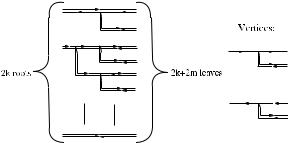
Dynamics of Bose-Einstein Condensates |
585 |
are drawn below). Graphs in Fm,k have 2k + 3m edges, 2k roots (the edges on the very left), and 2k + 2m leaves (the edges on the very right). It is possible to show that the number of different graphs in Fm,k is bounded by 24m+k .
The particular form of the graphs in Fm,k is due to the quantum mechanical nature of the expansion; the presence of a commutator in the collision operator (53) implies that, for every B in (55), we can choose whether to write the interaction on the left or on the right of the density. When we draw the corresponding vertex in a graph in Fm,k , we have to choose whether to attach it on the incoming or on the outgoing edge.
Graphs in Fm,k are characterized by a natural partial ordering among the vertices (v v if the vertex v is on the path from v to the roots); there is, however, no total ordering. The absence of total ordering among the vertices is the consequence of a rearrangement of the summands on the r.h.s. of (55); by removing the order between times associated with non-ordered vertices we significantly reduce the number of terms in the expansion. In fact, while (55) contains (m + k)!/ k! summands, in (57) we are only summing over 24m+k contributions. The price we have to pay is that the apparent gain of a factor 1/m! because of the ordering of the time integrals in (55) is lost in the new expansion (57). However, since the time integrations are already needed to smooth out singularities, and since they cannot be used simultaneously for smoothing and for gaining a factor 1/m!, it seems very difficult to make use of the apparent factor 1/m! in (55). In fact, we find that the expansion (57) is better suited for analyzing the cumulative space-time smoothing effects of the multiple free evolutions than (55).
Because of the pairing of the 2k trees, there is a natural pairing between the 2k roots of the graph. Moreover, it is also possible to define a natural pairing of the leaves of the graph (this is evident in Fig. 1); two leaves 1 and 2 are paired if there exists an edge e1 on the path from 1 back to the roots, and an edge e2 on the path from 2 to the roots, such that e1 and e2 are the two unmarked son-edges of the same vertex (or, if there is no unmarked sons in the path from 1 and 2 to the roots, if the two roots connected to 1 and 2 are paired).
For Λ Fm,k , we denote by E(Λ), V (Λ), R(Λ) and L(Λ) the set of all edges, vertices, roots and, respectively, leaves in the graph Λ. For every edge e E(Λ),
we introduce a three-dimensional momentum variable pe and a one-dimensional |
|||||||||
frequency variable αe . Then, denoting by γ0(k+m) |
and by J (k) |
the kernels of the |
|||||||
density γ0(k+m) and of the observable J (k) in Fourier space, the contribution KΛ,t |
|||||||||
in (57) is given by |
|
|
|
|
|
|
|
|
|
KΛ,t = |
|
|
|
dpedαe |
δ |
e v ±αe δ |
e v ±pe |
||
|
|||||||||
e E(Λ) |
αe − pe2 + iτe μe |
v V (Λ) |
|||||||
× exp |
−it |
τe (αe + iτe μe ) |
|
J (k)({pe }e R(Λ)) |
|||||
|
|
|
e R(Λ) |
|
|
|
|
|
|
× |
γ (k+m)( p |
e }e L(Λ) |
). |
|
|
|
(58) |
||
0 |
{ |
|
|
|
|
|
|||
586 |
Benjamin Schlein |
||
Here τe |
= ±1, according to the orientation of the edge e. We observe |
from (58) |
|
(k) |
, while |
||
that the momenta of the roots of Λ are the variables of the kernel of J |
|
||
the momenta of the leaves of Λ are the variables of the kernel of γ0(k+m) (this also explain why roots and leaves of Λ need to be paired).
The denominators (αe −pe2 +iτe μe )−1 are called propagators; they correspond to the free evolutions in the expansion (55) and they enter the expression (58) through the formula
|
itp2 |
∞ |
eit (α+iμ) |
e |
|
= −∞ dα |
|
|
α − p2 + iμ |
(here and in (58) the measure dα is defined by dα = d α/(2π i) where d α is the Lebesgue measure on R).
The regularization factors μe in (58) have to be chosen such that μfather = e= son μe at every vertex. The delta-functions in (58) express momentum and frequency conservation (the sum over e v denotes the sum over all edges adjacent to the vertex v; here ±αe = αe if the edge points towards the vertex, while ±αe = −αe
if the edge points out of the vertex, and analogously for ±pe).
An analogous expansion can be obtained for the error term ηn,t(k) in (56). The problem now is to analyze the integral (58) (and the corresponding integral for the error term). Through an appropriate choice of the regularization factors μe one can extract the time dependence of KΛ,t and show that
KΛ,t |
| ≤ |
Ck+mt m/4 |
|
|
dαe dpe |
|
|
|
δ |
e v ± |
αe δ |
e v ± |
pe |
|
|
|
|
|
|
|
|||||||||
| |
|
|
e E(Γ ) αe − pe2 v V (Γ ) |
|
|
|||||||||
|
|
× |
J (k)( p |
e }e R(Γ ) |
) |
γ (k+m) |
( |
|
p |
e }e L(Γ ) |
) |
|
|
(59) |
|
|
{ |
|
0 |
{ |
|
|
|
|
|
||||
where we introduced the notation x = (1 + x2)1/2.
Because of the singularity of the interaction at zero, we may be faced here with an ultraviolet problem; we have to show that all integrations in (59) are finite in the regime of large momenta and large frequency. Because of (46), we know that
the kernel γ0(k+m)({pe }e L(Λ)) in (59) provides decay in the momenta of the leaves. From (46) we have, in momentum space,
dp1 · · · dpn(p12 + 1) · · · (pn2 + 1)γ0(n)(p1, . . . , pn; p1, . . . , pn) ≤ Cn
for all n ≥ 1. Power counting implies that
|γ0(k+m)({pe }e L(Λ))| |
pe −5/2. |
(60) |
|
e L(Λ) |
|
Using this decay in the momenta of the leaves and the decay of the propagatorsαe − pe2 −1, e E(Λ), we can prove the finiteness of all the momentum and frequency integrals in (58). Heuristically, this can be seen using a simple power

588 |
|
|
|
Benjamin Schlein |
|
dαudαd dαw dpudpd dpw δ(αr = αu + αd − αw )δ(pr = pu + pd − pw ) |
|||
|
|
|pu|λ|pd |λ|pw |λ |
αu − pu2 αd − pd2 αw − pw2 |
|
≤ |
const |
(61) |
||
|
. |
|||
|pr |λ |
||||
Power counting implies that (61) can only be correct if λ > 2. On the other hand, to start the integration scheme we need λ < 5/2 (from (60) this is the decay in the momenta of the leaves, obtained from the a-priori estimates). It turns out that, choosing λ = 2 + ε for a sufficiently small ε > 0, (61) can be made precise, and the integration scheme can be completed.
After integrating all the frequency and momentum variables, from (59) we obtain that
|KΛ,t | ≤ Ck+mt m/4
for every Λ Fm,k . Since the number of diagrams in Fm,k is bounded by Ck+m, it follows immediately that
TrJ (k)ξm,t(k) ≤ Ck+mt m/4.
Note that, from (55), one may expect ξm,t(k) to be proportional to t m. The reason why we only get a bound proportional to t m/4 is that we effectively use part of the time integration to control the singularity of the potentials.
Note that the only property of γ0 used in the analysis of (58) is the estimate (46), which provides the necessary decay in the momenta of the leaves. However, since the a-priori bound (47) hold uniformly in time, we can use a similar argument to bound the contribution arising from the error term ηn,t(k) in (56) (as ex-
plained above, also ηn,t(k) can be expanded analogously to (57), with contributions associated to Feynman graphs similar to (58); the difference, of course, is that these
s |
|
[ |
] |
, while (58) only depends on |
|
contributions will depend on γ (k+n) for all s |
|
0, t |
|||
the initial data). Thus, we also obtain |
|
|
|
|
|
TrJ (k)ηn,t(k) |
≤ Ck+nt n/4. |
(62) |
|||
This bound immediately implies the uniqueness. In fact, given two solutions Γ1,t = {γ1(k),t }k≥1 and Γ2,t = {γ2(k),t }k≥1 of the infinite hierarchy (29), both satisfying the a- priori bounds (47) and with the same initial data, we can expand both in a Duhamel
series of order n as in (54). If we fix k ≥ 1, and consider the difference between γ1(k),t and γ2(k),t , all terms (55) cancel out because they only depend on the initial data.
Therefore, from (62), we immediately obtain that, for arbitrary (sufficiently smooth) compact k-particle operators J (k),
TrJ (k)(γ1(k),t − γ2(k),t ) ≤ 2Ck+nt n/4.
Dynamics of Bose-Einstein Condensates |
589 |
Since it is independent of n, the left side has to vanish for all t < 1/C4. This proves uniqueness for short times. But then, since the a-priori bounds hold uniformly in time, the argument can be repeated to prove uniqueness for all times.
References
1.R. Adami, F. Golse, and A. Teta, Rigorous derivation of the cubic NLS in dimension one. Preprint: Univ. Texas Math. Physics Archive. http://www.ma.utexas.edu, No. 05-211
2.M.H. Anderson, J.R. Ensher, M.R. Matthews, C.E. Wieman, and E.A. Cornell, Science 269, 198 (1995)
3.C. Bardos, F. Golse, and N. Mauser, Weak coupling limit of the N -particle Schrödinger equation. Methods Appl. Anal. 7, 275–293 (2000)
4.K.B. Davis, M.-O. Mewes, M.R. Andrews, N.J. van Druten, D.S. Durfee, D.M. Kurn, and W. Ketterle, Phys. Rev. Lett. 75, 3969 (1995)
5.L. Erdos˝ and H.-T. Yau, Derivation of the nonlinear Schrödinger equation from a many body Coulomb system. Adv. Theor. Math. Phys. 5(6), 1169–1205 (2001)
6.L. Erdos,˝ B. Schlein, and H.-T. Yau, Rigorous derivation of the Gross-Pitaevskii equation. Phys. Rev. Lett. 98(4), 040404 (2007)
7.L. Erdos,˝ B. Schlein, and H.-T. Yau, Derivation of the cubic non-linear Schrödinger equation from quantum dynamics of many-body systems. Invent. Math. 167(3), 515–614 (2007)
8.L. Erdos,˝ B. Schlein, and H.-T. Yau, Derivation of the Gross-Pitaevskii equation for the dynamics of Bose-Einstein condensate. Ann. Math. (to appear). Preprint arXiv:math-ph/0606017
9.E.H. Lieb and R. Seiringer, Proof of Bose-Einstein condensation for dilute trapped gases. Phys. Rev. Lett. 88(17), 170409 (2002)
10.E.H. Lieb, R. Seiringer, and J. Yngvason, Bosons in a trap: A rigorous derivation of the GrossPitaevskii energy functional. Phys. Rev A 61(4), 043602 (2000)
11.H. Spohn, Kinetic equations from Hamiltonian dynamics. Rev. Mod. Phys. 52(3), 569–615 (1980)

Locality Estimates for Quantum Spin Systems
Bruno Nachtergaele and Robert Sims
Abstract We review some recent results that express or rely on the locality properties of the dynamics of quantum spin systems. In particular, we present a slightly sharper version of the recently obtained Lieb-Robinson bound on the group velocity for such systems on a large class of metric graphs. Using this bound we provide expressions of the quasi-locality of the dynamics in various forms, present a proof of the Exponential Clustering Theorem, and discuss a multi-dimensional Lieb-Schultz- Mattis Theorem.
1 Introduction
Locality is a fundamental property of all current physical theories. Sets of observables can be associated with points or bounded regions in space or space-time and a relativistic dynamics will preserve this structure [7]. How the locality property manifests itself mathematically in important situations continues to be an active topic of investigation [12].
There is a wide range of important physical systems, however, which we prefer to describe by very effective non-relativistic quantum theories with Hamiltonian dynamics. Even if the Hamiltonian has only finite-range interactions, the dynamics it generates generally does not preserve locality, i.e., there is no strict equivalent to the finite speed of light. However, locality still holds in an approximate sense, and there is an associated finite velocity, which is sometimes referred to as the group velocity. We call it the Lieb-Robinson velocity since Lieb and Robinson were the
Bruno Nachtergaele
Department of Mathematics, University of California, Davis, CA 95616, USA, e-mail: bxn@math.ucdavis.edu
Robert Sims
Department of Mathematics, University of Arizona, Tucson, AZ 85721, USA, e-mail: rsims@math.arizona.edu
V. Sidoraviciusˇ (ed.), New Trends in Mathematical Physics, |
591 |
© Springer Science + Business Media B.V. 2009 |
|
592 |
Bruno Nachtergaele and Robert Sims |
first to prove its existence and to obtain a bound for it [14]. They proved that to a high degree of accuracy locality is preserved by quantum spin dynamics in the sense that any local observable evolved for a time t > 0 remains localized in a region of space with diameter proportional to t , up to an arbitrarily small correction. This also means that spatial correlations between observables separated by a distance d cannot be established faster than a time of order d.
The fundamental issue of locality may be sufficient motivation to extend the Lieb-Robinson bounds to more general situations, but there are other good reasons to try to generalize their result and to improve the estimates they obtained. As we will discuss below, locality, or the approximate locality of the dynamics, has been shown to be responsible for a considerable number of other important properties relevant for models of many-body systems. In many situations, however, the implications of locality have yet to be fully explored.
We will begin this note by presenting a short proof of the new Lieb-Robinson bounds obtained successively in [18, 10], and [21]. This improved result we give below sharpens the bounds previously obtained in that the prefactor now only grows as the smallest surface area of the supports of the local observables. We do this in Sect. 2. An application where this surface area dependence, rather than volume dependence, is important can be found in [5].
In Sect. 3, we present two perspectives on how Lieb-Robinson bounds may be used to provide explicit estimates on the local structure of the time evolution. As a consequence, one easily derives bounds on, for example, multiple commutators and the rate at which spatial correlations can be established in normalized product states.
Section 4 discusses the so-called Exponential Clustering Theorem. In the relativistic context it has been known for a long time that a gap in the spectrum above the vacuum state implies exponential decay of spatial correlations in that state [3, 23, 6]. That a similar result should hold in the non-relativistic setting such as quantum spin systems was long expected and taken for granted by theoretical physicists [24]. In [9], Hastings proposed to use Lieb-Robinson bounds to obtain such a result and a complete proof was recently given in [18, 10].
As a final application of these locality bounds, we describe a new proof of the Lieb-Schultz-Mattis theorem, see [9, 19], in Sect. 5. These results can be traced back to [9] where Hastings introduced a new way to construct and analyze variational states for low-lying excitations of gapped Hamiltonians. He developed a notion of a quasi-adiabatic evolution [11] which he then used to present a multi-dimensional analogue of the celebrated Lieb-Schultz-Mattis theorem [15]. Such a theorem is applicable, for example, to the standard spin-1/2, anti-ferromagnetic Heisenberg model and yields an upper bound on the first excited state of order c(log L)/L for systems of size L. His arguments rely on Lieb-Robinson bounds and the Exponential Clustering Theorem in an essential way, and we have recently obtained a rigorous proof of this result which holds in a rather general setting, see [19].
We expect that the ideas currently emerging from recent applications of LiebRobinson bounds will continue to lead to interesting new results for quantum spin systems in the near future.
Locality Estimates for Quantum Spin Systems |
593 |
2 Lieb-Robinson Bounds |
|
The first proof of locality bounds in the context of quantum spin systems appeared in 1972 in a paper by Lieb and Robinson [14]. They proved a bound on the group velocity corresponding to the dynamics generated by a variety of short range Hamiltonians. In a series of works [18, 10], and [21], these estimates have been generalized, and the proof we provide below, see Theorem 1, illustrates many of the new insights which have recently been developed.
The result stated in Theorem 1 below differs from that which may be found in [14] in two important ways. First, the new proof does not require the use of the Fourier transform, and therefore, it extends to models defined on sets without an underlying lattice structure. These results may be of interest to those who wish to study quantum spin systems in the context of quasi-crystals or in the study of circuits for quantum computation. Second, and most importantly, the constants which appear in our bound do not depend on the dimensions of the underlying, single-site Hilbert spaces. This opens up the possibility of applying them to models with an infinite-dimensional Hilbert space, such as lattice oscillators [22].
The basic set up in this theory concerns quantum spins systems, in particular, a finite or infinite number of spins labeled by x V . A finite dimensional Hilbert space Hx is assigned to each site x V . These may represent the spin of an electron, photon, or an atom. In other contexts, these states may represent the ground state and first exited state of an atom or a molecule. More abstractly, these systems may, for example, model a collection qubits, the basic units of quantum information theory and quantum computation.
If the set V is finite, the Hilbert space of states is given by HV = |
x V Hx . |
For each spin x, the observables are the complex nx × nx matrices, Mnx , where |
|
nx = dim(Hx ). In this context, the algebra of observables for the whole system is |
|
AV = x V Mnx .
The locality results we wish to describe pertain to observables with finite support. Here, the support of an observable is understood as follows. If X V , we write AX = x X Mnx . By identifying A AX with A 1l AV , we have that AX AV . The support of an observable A AV in the minimal set X V for which A = A 1l with A AX .
For infinite V , the algebra of observables is the completion of the algebra of local observables given by
AV = AX
X V
where the union is over all finite X V .
To describe the models we wish to investigate, we must first define interactions, local Hamiltonians, and the corresponding dynamics. An interaction is a map Φ from the set of subsets of V to AV with the property that Φ(X) AX and Φ(X) = Φ(X) for all finite X V . A quantum spin model is defined by a family of local Hamiltonians, parametrized by finite subsets Λ V , given by
594 Bruno Nachtergaele and Robert Sims
HΛΦ = Φ(X). |
(1) |
X Λ |
|
For notational convenience, we will often drop the dependence of HΛΦ on Φ. The dynamics, or time evolution, generated by a quantum spin model is the one-parameter group of automorphisms, {τtΛ}t R, defined by
τ Λ(A) |
= |
eit HΛ Ae−it HΛ , A |
|
AΛ, |
(2) |
t |
|
|
|
which is always well defined for finite sets Λ. In the context of infinite systems, a boundedness condition on the interaction is required in order for the finite-volume dynamics to converge to a strongly continuous one-parameter group of automorphisms on AV .
The locality results we prove in Theorem 1 are valid for a large class of interactions. To describe this class precisely, we first put a condition on the set V , which is relevant only in the event that V is infinite. We assume that the set V is equipped with a metric d and that there exists a non-increasing function F : [0, ∞) → (0, ∞) for which:
(i) F is uniformly integrable over V , i.e.,
F = sup |
F (d(x, y)) < ∞, |
(3) |
||
x V y V |
|
|
|
|
and |
|
|
|
|
(ii) F satisfies |
|
|
|
|
C = sup |
F (d(x, z))F (d(z, y)) |
< ∞. |
(4) |
|
|
|
|||
|
F (d(x, y)) |
|||
x,y V z V |
|
|
|
|
Given such a set V , it is easy to see that for any F which satisfies (i) and (ii) above, then the family of functions Fa , for a ≥ 0, defined by
|
Fa (x) = e−ax F (x), |
(5) |
|||
also satisfy i) and ii) with |
Fa ≤ F |
and Ca ≤ C. In this context, we define the |
|||
set Ba (V ) to be those interactions Φ on V which satisfy |
|
||||
|
|
|
Φ(X) |
|
|
Φ |
a = sup |
|
|
< ∞. |
(6) |
|
Fa (d(x, y)) |
||||
|
x,y V X x,y |
|
|||
The Lieb-Robinson bounds we will prove are valid for all Φ Ba (V ) with a ≥ 0. Simply stated, these results correspond to estimates of the form
[τtΛ(A), B] ≤ c(A, B)e−μ(d(A,B)−vΦ |t |), |
(7) |
where A and B are local observables, τtΛ(·) is the time evolution corresponding to a finite volume Hamiltonian generated by an interaction Φ Ba (V ), and d(A, B)
596 Bruno Nachtergaele and Robert Sims
produces an analogous bound with the factor e2 Φ a Ca |t | − 1 replaced by e2 Φ a Ca |t |. In the case of empty intersection and for small values of |t |, (13) is a better and
sometimes useful estimates than the obvious bound [τt (A), B] ≤ 2 |
A |
B , valid |
|||||||
for all t R. |
|
|
|
|
|
|
|
|
|
Next, if Φ Ba (V ) for some a > 0, then one has the trivial estimate that |
|||||||||
Da (X, Y ) ≤ |
F0 Φ a min(|∂Φ X|, |∂Φ Y |)e−ad(X,Y ). |
|
(15) |
||||||
Clearly then, we have that |
|
|
|
|
|
|
|
||
[τtΛ(A), B] ≤ |
2 A |
B |
F0 |
min(|∂Φ X|, |∂Φ Y |)e−a[d(X,Y )− |
2 Φ a Ca |
|t |], (16) |
|||
|
|
|
|
a |
|||||
|
Ca |
|
|
||||||
which corresponds to a bound on the velocity of propagation given by |
|
||||||||
|
|
|
|
inf |
2 Φ a Ca |
. |
|
|
(17) |
|
|
|
|
|
|
|
|||
|
|
|
vΦ ≤ a>0 |
a |
|
|
|
||
Next, we observe that for fixed local observables A and B, the bounds above, (13) and (16), are independent of the volume Λ V ; given that Λ contains the supports of both A and B. Furthermore, we note that these bounds only require that one of the observables has finite support; in particular, if |X| < ∞ and d(X, Y ) > 0, then the bounds are valid irrespective of the support of B.
Proof (of Theorem 1). To prove (13), we will provide an estimate on the quantity
C |
B |
(Z |
; |
t ) |
= |
sup |
[τtΛ(A), B] |
, |
(18) |
|
|||||||||
|
|
|
A AZ |
A |
|
||||
|
|
|
|
|
|
|
|
|
|
where B is a fixed observable with support in Y , and the subset Z Λ we regard as arbitrary. Introduce the function
f (t ) = τtΛ(τ−Xt (A)), B , |
(19) |
where A and B are as in the statement of the theorem. Due to the strict locality of the Hamiltonian HX , as defined e.g. in (12) and the fact that the observable A AX , we have that supp(τ−Xt (A)) X for all t R. It is straight forward to verify that
f (t ) |
= |
i |
τ Λ(Φ(Z)), f (t ) |
− |
i |
|
τ Λ(τ X (A)), |
τ Λ(Φ(Z)), B . |
|
|
|
t |
Z SΛ(X) |
t |
−t |
t |
|||
|
|
|
Z SΛ(X) |
|
|
|
(20) |
||
|
|
|
|
|
|
|
|
|
|
Since the first term in (20) is norm preserving, we find that |
|
||||||||
|
|
|
|
|
|
|
|
t |
|
[τtΛ(τ−Xt (A)), B] ≤ [A, B] + 2 A |
|
0 |
[τsΛ(Φ(Z)), B] ds. (21) |
||||||
|
|
|
|
|
Z S(X) |
|
|
|
|
The inequality (21) and the fact that |
τ−Xt (A) |
= A |
together imply that |
||||||

598 |
Bruno Nachtergaele and Robert Sims |
3 Quasi-Locality of the Dynamics
The Lieb-Robinson bounds of Theorem 1 imply that the dynamics of quantum lattice systems, those generated by short range interactions, are quasi-local in the sense that the diameter of the support of any evolved local observable does not grow faster than linearly with time, up to an arbitrarily small error. There are at least two interesting ways to give precise meaning to this quasilocality property of the dynamics. In the first, one shows that the time-evolved observable can be well-approximated in norm by one with a strictly local support. This is achieved by the quantum version of integrating out the variables in the complement of a ball with a radius proportional to time. In the second, we show that to compute the dynamics up to a time t > 0, one can replace the Hamiltonian with a local Hamiltonian supported in a ball of radius proportional to t . Clearly, the net result is the same: the support of observables evolved with approximate dynamics remains contained in the ball where the local Hamiltonian is supported. After presenting the details of these two approaches, we conclude this section with a few interesting applications that immediately follow from quasi-locality.
As in the previous section, we will work with an interaction Φ Ba (V ) with a > 0. For the purpose of the discussion below, we will consider a finite subset Λ V and restrict our attention to the dynamics τtΛ(·) generated by the finite volume Hamiltonian HΛ as defined in (1); our bounds will be independent of the volume Λ. For any X Λ we will denote by Xc = Λ \ X.
In the first approach to obtaining a local approximation with support contained in X Λ, one takes the normalized partial trace over the Hilbert space associated with Xc. In order to estimate the norm difference it is convenient to calculate the partial trace as an integral over the group of unitaries [4]. Given an arbitrary observable A AΛ and a set X Λ, define
A Xc = U AU μ(dU ), (30)
U (Xc )
where U (Xc) denotes the group of unitary operators over the Hilbert space HXc and μ is the associated, normalized Haar measure. It is easy to see that for any A AΛ, the quantity A Xc has been localized to X in the sense that A Xc AX . Moreover, the difference may be written in terms of a commutator, i.e. as
A Xc − A = |
U (Xc ) U [A, U ]μ(dU ). |
(31) |
||||||
To localize the dynamics, let A AX |
and fix |
> |
0. Based on our estimates in |
|||||
|
Λ |
|
||||||
Theorem 1, we approximate the support of |
τt (A) with a time-dependent ball |
|
||||||
Bt ( , A) = x Λ : d(x, X) ≤ |
2 Φ a Ca |
|t | + . |
(32) |
|||||
|
a |
|
||||||
For any unitary U U (Bt ( , A)c), we clearly have that
Locality Estimates for Quantum Spin Systems |
|
|
599 |
d(X, supp(U )) ≥ |
2 Φ a Ca |
|t | + , |
(33) |
|
|||
a |
and therefore, using (31) above and our bound (16), we immediately conclude that
τtΛ(A) − τtΛ(A) Bt ( ,A)c ≤ |
c |
τtΛ(A), U |
μ(dU ) |
||||
|
U (Bt ( )) |
|
|
|
|
||
≤ |
2 A |∂Φ X| |
|
F |
0 |
e−a . |
(34) |
|
Ca |
|||||||
|
|
|
|||||
The tolerance > 0 can be chosen to optimize estimates.
In the second approach, one shows that only those terms in the Hamiltonian supported in BT ( , A) contribute significantly to the time evolution of A up to time T [21]. Again, we consider the finite volume dynamics applied to a local observable A AX . Fix > 0, T > 0, and consider the ball BT ( , A) as defined in (32) above. The estimate
τ Λ(A) |
− |
τ BT ( ,A) |
(A) |
≤ |
A |
F0 |∂Φ X| |
(Ca |
+ |
Fa )e−a , |
(35) |
|
Ca2 |
|||||||||
t |
t |
|
|
|
|
|
valid for all |t | ≤ T , readily follows from the results in [21]. In fact, the proof of (35) uses the following basic estimate, see e.g. Lemma 3.3 in [21],
Lemma 2. Let Φ Ba (V ) with a > 0 and take a finite subset Λ V . If the
finite volume Hamiltonian is written as the sum of two self-adjoint operators, HΛ = HΛ(1) + HΛ(2), and for i = 1, 2, τt(i)(·) denotes the dynamics corresponding to HΛ(i),
then the following estimate is valid:
|t |
τtΛ(A) − τt(1)(A) ≤ HΛ(2), τs(1)(A) ds, (36)
0
for any observable A and t R.
To apply Lemma 2 in the context discussed above, we write the local Hamiltonian as the sum of two terms:
HΛ = |
Φ(Z) + |
|
|
|
Φ(Z) = HΛ(1) + HΛ(2). |
(37) |
|
Z Λ: |
|
|
Z Λ: |
|
|
|
|
Z /SΛ(BT ( ,A)) |
Z SΛ(BT ( ,A)) |
|
|
||||
Recall that for any X Λ, we defined SΛ |
(X), the surface across X in Λ, with (8). |
||||||
(2) |
|
|
|
|
|||
Dropping the surface terms comprising HΛ |
above, decouples the dynamics, i.e., |
||||||
τt(1)(A) = τtBT ( ,A)(A), and we find that for any |t | ≤ T , |
|
||||||
τtΛ(A) − τtBT ( ,A)(A) |
≤ |
Z Λ: |
|
0 |
|t | |
Φ(Z), τsBT ( ,A)(A) ds. |
(38) |
|
|
|
|
|
|
|
|
|
|
Z SΛ(BT ( ,A)) |
|
|
|
|
|
600 |
Bruno Nachtergaele and Robert Sims |
For each of the terms on the right hand side above, the Lieb-Robinson estimates imply that
|
|
2 Φ(Z) A |
|
|
Φ(Z), τ BT ( ,A)(A) |
≤ |
|
e2 Φ a Ca |s| |
Fa (d(x, z)). (39) |
|
||||
s |
Ca |
z Z x ∂Φ X |
||
|
|
|
|
|
Careful consideration of the combinatorics of these sums, exactly as done in [21], yields (35) as claimed.
It is interesting to ask about locality bounds for complex times. For one-dimens- ional systems with finite range interactions, Araki proved that the support does not grow faster than an exponential in |z|, where z is the complex time [2, Theorem 4.2]. In other words, the complex time evolution
τz[−R,R](A) = eizHΛ Ae−izHΛ
can be approximated by τz[−N,N ](A) with small error, uniformly in R, as long as log |z| ≤ cN , for a suitable constant c. For stochastic dynamics of classical particle systems, good locality bounds that are very similar to Theorem 1 are known [16, Theorem 4.20]. Since these classical models with stochastic dynamics can be thought of as quantum systems, generated by particular Hamiltonians and evolving with purely imaginary times, this may indicate that the general result, which allows for no more than logarithmic growth of |z|, should not be considered the final word on this issue in regards to specific models of interest.
The quasi-locality formulation of the Lieb-Robinson bounds makes it easy to derive bounds on double and higher order commutators of the form
[τt1 (A), [τt2 (B), τt3 (C]].
Such commutators remain small in norm as long as t1, t2, and t3 are such that the intersection of the time-dependent “quasi-supports” remains empty. That is whenever t1, t2, t3 R are such that
Bt1 ( , A) ∩ Bt2 ( , B) ∩ Bt3 ( , C) = .
Another immediate application of the quasi-locality property is a bound on the rate at which spatial correlations can be created by the dynamics starting from a product state. In [21], we proved the following.
Theorem 3. Let a > 0, Φ Ba (V ), and take Ω to be a normalized product state. Given X, Y Λ with d(X, Y ) > 0 and local observables A AX and B AY , the estimate
| τt (AB) − τt (A) τt (B) | ≤ 4 A B F (|∂Φ X| + |∂Φ Y |)Ga (t )e−ad(X,Y )
(40) is valid for all t R. Here, for any observable A, the expectation value of A in the state Ω is denoted by A = Ω, AΩ , and the function
Locality Estimates for Quantum Spin Systems |
601 |
G |
(t ) |
= |
|
Ca + Fa |
Φ |
|
|t | |
e2 Φ a Ca |s|ds. |
(41) |
|
|
|
|||||||
a |
|
|
Ca |
a |
0 |
|
|
||
4 Exponential Clustering
As a second application of these locality bounds, we will present a proof of the Exponential Clustering Theorem, see Theorem 4 below, which improves on the estimates found in [18], see also [10]. The proof of exponential clustering demonstrates that models with a spectral gap above the ground state energy necessarily exhibit exponential decay of spatial correlations in their ground state. Such results have recently appeared in a variety of contexts, e.g. [18, 10]. Using valence bond states, as is done in [17], one can easily construct gapless models with exponentially decaying ground state correlations indicating that, in general, there is no converse to Theorem 4.
In the finite volume, the notion of a gapped Hamiltonian is clear. If the system is infinite, we express the gap condition in terms of the limiting dynamics, the existence of which is guaranteed by the Lieb-Robinson bounds as discussed above, by considering a representation of the system on a Hilbert space H . This means that there is a representation π : AV → B(H ), and a self-adjoint operator H on H such that
π(τt (A)) = eit H π(A)e−it H , A AV . |
(42) |
We will assume that the representative operator H is non-negative and that there exists a vector Ω H for which H Ω = 0. We say that the system has a spectral gap in the representation if there exists δ > 0 such that spec(H ) ∩ (0, δ) = . In this case, the spectral gap, γ , is defined by
γ = sup{δ > 0 | spec(H ) ∩ (0, δ) = }. |
(43) |
Let P0 denote the orthogonal projection onto ker H . From now on, we will work in this representation and simply write A instead of π(A).
Theorem 4 (Exponential Clustering). Let a > 0 and take Φ Ba (V ). Suppose that the dynamics corresponding to Φ on V can be represented by a Hamiltonian H with a gap γ > 0 above the ground state energy, as described above. Let Ω be a normalized ground state vector for H ; i.e. satisfy H Ω = 0 with Ω = 1. Then, there exists a constant μ > 0 such that for any local observables A AX and B AY with X, Y V and d(X, Y ) > 0 satisfying P0BΩ = P0B Ω = 0, the bound
| Ω, Aτib(B)Ω | ≤ C(A, B, γ )e−μd(X,Y )(1+ |
γ 2b2 |
|
|||
|
) |
(44) |
|||
4μ2d(X,Y )2 |
|||||
is valid for all non-negative b satisfying 0 ≤ bγ ≤ 2μd(X, Y ). One may take |
|
||||
μ = |
aγ |
|
|
(45) |
|
|
, |
|
|
||
4 Φ a Ca + γ |
|
|
|||
602 |
|
|
|
|
Bruno Nachtergaele and Robert Sims |
||
as well as a constant |
|
|
|
|
|
|
|
|
|
|
|
|
|
|
|
C(A, B, γ ) = A B 1 + |
|
1 |
|
+ |
2 F0 |
min(|∂Φ X|, |∂Φ Y |) . |
(46) |
μd(X, Y ) |
π Ca |
||||||
Note that in the case of a non-degenerate ground state, the condition on B is
equivalent to Ω, BΩ = 0. In this case, the theorem with b = 0 becomes |
|
| Ω, ABΩ − Ω, AΩ Ω, BΩ | ≤ C(A, B, γ )e−μd(X,Y ), |
(47) |
which is the standard (equal-time) correlation function. For small b > 0, the estimate (44) can be viewed as a perturbation of (47). Moreover, for b > 0 large, there is a trivial bound
| Ω, Aτib(B)Ω | ≤ A B e−bγ . |
(48) |
Proof. (of Theorem 4) We will follow very closely the proof which appears in [18] and refer to it whenever convenient. Consider the function f given by
|
|
∞ |
|
f (z) = Ω, Aτz(B)Ω = |
γ |
eizE d A Ω, PE BΩ , |
(49) |
where we have used the spectral theorem and the fact that B projects off the ground state. It is clear that the function f defined in (49) is analytic in the upper half plane and has a continuous (and bounded) boundary value on the real axis. The quantity we wish to bound corresponds to f (ib) for b > 0. The case b = 0 will follow by a limiting argument.
Since the boundary value of f on R is continuous, one may show by a limiting argument that for any T > b,
f (ib) = |
1 |
|
f (z) |
(50) |
|
|
ΓT |
|
dz, |
||
2π i |
z − ib |
||||
where ΓT is the semi-circular contour from −T to T (on the real axis) into the upper half plane. As is shown in [18], the fact that the Hamiltonian is gapped, see also (49), implies that the integral over the circular part of the contour vanishes in the limit as T → ∞, and therefore we have the bound
|
1 |
T |
|
f (t ) |
|
||
| Ω, Aτib(B)Ω | = |f (ib)| ≤ lim sup |
|
|
(51) |
||||
|
|
|
|
|
dt . |
||
2π i |
−T |
t |
− |
ib |
|||
T →∞ |
|
|
|
|
|
||
The proof is then complete once we estimate this integral over the real line. While this inequality is true for any value of b > 0, to get the desired estimate, we will have to choose b > 0 sufficiently small; see the comments following (64) below.
Let α > 0. We will choose this free parameter later. Observe that one may write
f (t ) = e−αb2 f (t )e−αt 2 + f (t ) eαb2 − e−αt 2 . |
(52) |
Locality Estimates for Quantum Spin Systems |
603 |
Clearly then, the integral we wish to bound, the one on the right hand side of (51) above, can be estimated by
e−αb2 |
1 |
T |
f (t )e−αt 2 |
dt |
+ |
e−αb2 |
1 |
T |
f (t )(eαb2 − e−αt 2 ) |
dt . (53) |
||||
|
−T |
|
|
−T |
|
|||||||||
|
2π i |
t |
− |
ib |
|
2π i |
t |
− |
ib |
|||||
|
|
|
|
|
|
|||||||||
We will bound the absolute value of each of the integrals appearing in (53) separately; the prefactor e−αb2 will be an additional damping made explicit by the choice of α.
To bound the first integral appearing in (53), we further divide the integrand into two terms. Note that
|
|
|
f (t )e−αt 2 |
= Ω, τt (B)AΩ e−αt 2 + Ω, [A, τt (B)]Ω e−αt 2 . |
(54) |
|||||||||||||
By the spectral theorem, we have that |
|
|
|
|
|
|
|
|
|
|
|
|||||||
|
1 T |
Ω, τt (B)AΩ e−αt 2 |
dt |
= |
|
∞ 1 |
T |
e−it E e−αt 2 dt d |
PE B |
Ω, AΩ |
, |
|||||||
|
|
|
|
|
|
|
|
|||||||||||
2π i |
|
|
|
|
2π i |
|
||||||||||||
−T |
t |
− |
ib |
γ |
|
−T |
t |
− |
ib |
|
|
|
|
|||||
|
|
|
|
|
|
|
|
|
|
|
|
(55) |
||||||
|
|
|
|
|
|
|
|
|
|
|
|
|
|
|
|
|
||
where we have used now that B Ω is also orthogonal to the ground state. Applying Lemma 5, stated below, to the inner integral above, we have that
|
1 |
T e−it E e−αt 2 |
|
1 |
∞ |
bw |
|
(w+E)2 |
|
1 |
γ 2 |
||||
Tlim |
|
|
|
|
|
dt = |
2√ |
|
e− |
|
e− |
4α |
dw ≤ |
|
e− 4α , (56) |
2π i |
|
t |
− |
ib |
|
2 |
|||||||||
−T |
π α |
|
|
||||||||||||
→∞ |
|
|
|
|
|
|
0 |
|
|
|
|
|
|
||
where for the final inequality above we used that E ≥ γ > 0, α > 0, and b > 0. From this we easily conclude that
lim sup |
1 |
T |
Ω, τt (B)AΩ e−αt 2 |
dt |
≤ |
A |
B |
e− γ4α2 . |
(57) |
||
|
|
|
|
2 |
|||||||
T →∞ |
2π i |
−T |
t |
− |
ib |
|
|
|
|||
|
|
|
|
|
|
|
|
|
|||
For the integral corresponding to the second term in (54), it is easy to see that
1 T |
Ω, [A, τt (B)]Ω e−αt 2 |
dt |
≤ |
1 ∞ |
[A, τt (B)] e−αt 2 dt, (58) |
||||
2π i |
|
|
2π |
|
|||||
−T |
t |
− |
ib |
−∞ |
t |
||||
|
|
|
|
|
|
| | |
|||
where we have taken advantage of the fact that b > 0. To complete our estimate, we will introduce another free parameter s > 0. Here we use the Lieb-Robinson bound, Theorem 1, for times |t | ≤ s and a basic norm estimate otherwise. The result is that the right hand side of (58) is bounded from above by
2 |
A B |
A B |
2 |
|
||||
|
|
Da (X, Y )(e2 Φ a Ca s − 1) + |
s√ |
|
|
e−αs . |
(59) |
|
π |
Φ a Ca |
|||||||
π α |
||||||||
This completes the bound of the first integral appearing in (53).
Using again the spectral theorem, the second integral in (53) may be written as

604 Bruno Nachtergaele and Robert Sims
|
∞ 1 |
T |
eit E (eαb2 − e−αt 2 ) |
dt d |
A Ω, P |
|
BΩ |
|
. |
(60) |
|||
|
|
|
|
|
|
||||||||
|
2π i |
|
|
|
|||||||||
γ |
−T |
t |
− |
ib |
|
|
E |
|
|
|
|||
|
|
|
|
|
|
|
|
|
|
|
|||
As is described in detail in [18], we find that for E ≥ γ and α chosen such that
γ ≥ 2αb, |
1 T |
|
eit E |
2 |
2 |
|
1 |
|
γ 2 |
|
||||
Tlim |
|
|
|
|
|
(eαb |
|
− e−αt |
)dt ≤ |
|
e− |
|
, |
(61) |
|
|
|
|
|
|
|
4α |
|||||||
2π i |
−T |
t |
− |
ib |
|
2 |
||||||||
→∞ |
|
|
|
|
|
|
|
|
|
|
|
|
||
which produces an estimate (one analogous to the bound in (57) above) for (60). All of our estimates above combine to demonstrate that the right hand side of
(51) is bounded by
|
γ 2 |
|
2Da (X, Y ) |
|
1 |
|
2 |
||||||||
|
e− 4α + |
|
|
e−αs |
|||||||||||
A B |
|
|
|
|
(e2 Φ a Ca s − |
1) + |
s√ |
|
(62) |
||||||
|
π Φ a Ca |
||||||||||||||
|
π α |
||||||||||||||
if α satisfies γ ≥ 2αb. The choice α = γ /2s yields: |
|
|
|
|
|
|
|||||||||
|
|
|
|
|
|
|
|
2Da (X, Y ) |
|
|
|||||
A |
B e− γ2s |
1 |
+ |
|
2 |
|
|
e(2 Φ a Ca + γ2 )s |
(63) |
||||||
π γ s + |
|
||||||||||||||
|
|
|
|
π Φ a Ca |
|
|
|
|
|
|
|||||
As is demonstrated in (15), Da (X, Y ) decays exponentially as e−ad(X,Y ). In this case, if we choose s to be the solution of the equation
s(2 Φ a Ca + γ /2) = ad(X, Y ), |
(64) |
then we have proven the result. Notice that we have chosen α in terms of s, which is defined independently of b, thus the condition γ ≥ 2αb will be satisfied for sufficiently small b > 0.
In our proof of the Exponential Clustering Theorem above, we used several times the following useful fact, a proof of which appears in [18].
Lemma 5. Let E R, α > 0, and z C+ = {z C : Im[z] > 0}. One has that
|
1 |
T |
eiEt e−αt 2 |
dt = |
1 |
∞ |
iwz |
e− |
(w−E)2 |
|
|||
Tlim |
|
|
|
|
|
2√ |
|
e |
|
4α dw. |
(65) |
||
2π i |
|
t |
− |
z |
|
||||||||
−T |
π α |
|
|||||||||||
→∞ |
|
|
|
|
|
|
0 |
|
|
|
|
||
Moreover, the convergence is uniform for z C+.
5 The Lieb-Schultz-Mattis Theorem
As a final application of these locality bounds, in particular both Theorem 1 and Theorem 4, we were recently able to provide a rigorous proof the Lieb-Schultz- Mattis theorem, see [20], which is valid in arbitrary dimensions. In this section, we will discuss this result and outline the ideas which motivate our proof.
Locality Estimates for Quantum Spin Systems |
605 |
5.1 The Result and Some Words on the Proof |
|
The classical Lieb-Schultz-Mattis Theorem (LSM), [15], concerns the spin-1/2, anti-ferromagnetic Heisenberg chain. This model is defined through a family of
Hamiltonians HL, acting on the Hilbert space H[1,L] = |
x [1,L] C2, with the form |
||
HL = |
L−1 |
|
|
Sx · Sx+1. |
|
(66) |
|
|
x=1 |
|
|
Here, for each integer x [1, L], the spin vectors Sx have components |
|
||
Sxj = 1l · · · 1l Sj 1l · · · 1l, |
j = 1, 2, 3, |
(67) |
|
where Sj is the corresponding spin-1/2 (Pauli) matrix acting on the x-th factor of H[1,L]. The LSM Theorem may be stated as follows.
Theorem 6. (LSM, 1961) If the ground state of HL is unique, then the gap in energy between the ground state and the first excited state is bounded by C/L.
A further result by Lieb and Mattis in 1966, [13], verified that under certain conditions, for example when L is even, the main assumption in the LSM Theorem, specifically the uniqueness of the ground state, is indeed satisfied. Almost twenty years later, the LSM Theorem was generalized to encompass a variety of other one (and quasi-one) dimensional models by Affleck and Lieb in [1]. In particular, this result applies to those chains of even length with spins having arbitrary half-integer magnitude. Note: Here and in the rest of this section the term half-integer, or halfintegral, refers to one-half of a positive odd integer, i.e., an element of the set N + 1/2.
For models to which the LSM Theorem applies, one expects that the excitation spectrum corresponding to the thermodynamic limit has no gap above the ground state energy. It is interesting to note that the predictions of Haldane [8] suggest that such a result is rather sensitive to the type of interaction terms. In fact, the spin- 1, anti-ferromagnetic Heisenberg chain is predicted to have a robust gap above the ground state energy in the thermodynamic limit.
In a work of 2004, see [9], Hastings argued that a higher dimensional analogue of the LSM Theorem could be proven using the improved locality bounds which have recently been established. We will now summarize these ideas and indicate how they may be implemented to demonstrate a rigorous proof of this theorem.
The multi-dimensional LSM Theorem, stated as Theorem 7 below, is valid for a large class of models; a detailed proof of this is contained in [20]. For simplicity of presentation in this review article, we will restrict our attention to the spin-1/2, Heisenberg anti-ferromagnet, however, our general assumptions are discussed in Sect. 5.2.4. In ν dimensions, the model of interest is defined on subsets VL Zν in analogy to (66) above, i.e. one considers Hamiltonians

606 Bruno Nachtergaele and Robert Sims
HL = |
Sx · Sy |
(68) |
|
x,y VL: |
|
|
|x−y|=1 |
|
acting on the Hilbert space HVL = |
x VL C2. It is easy to state the new result. |
|
Theorem 7. If the ground state of HL is non-degenerate, then the gap, γL, above the ground state energy satisfies
γL ≤ C |
log(L) |
(69) |
L . |
The logarithmic correction which appears in Theorem 7, in contrast to the original result of Theorem 6, seems to be an inevitable consequence of the locality bounds we incorporate in our proof. It is an interesting open question to determine whether or not there is a class of models, in dimensions ν > 1, for which one can prove such a bound without the logarithmic correction.
In essense, Theorem 7 is proven using a variational argument. Letting ψ0 denote the unique, normalized ground state, we know that for any normalized vector ψ1 with | ψ0, ψ1 | = 1, the bound
0 < γ |
≤ |
ψ1, (H − E0)ψ1 |
(70) |
|
1 − | ψ0, ψ1 |2 |
||||
|
|
is always valid. Here we have dropped the dependence of all quantities on the length scale L. From this perspective, there are only three steps necessary to prove the desired result. First, we must construct a normalized trial state ψ1, as indicated above. Next, we must estimate the difference in the energy corresponding to ψ1 and E0. Lastly, we must ensure that the inner product | ψ0, ψ1 | remains sufficiently small.
This method of proof is complicated by the fact that the ground state is virtually unknown, and therefore the means by which one should construct a trial state is not a priori clear. Inspiration for the construction of our variational state comes from the work of Hastings, again see [9], in which he proposes to consider the ground state of a modified Hamiltonian, Hθ , where the interactions in a given hyperplane have been twisted by an angle of θ ; more on this below. The ground state of this modified Hamiltonian may be regarded as the solution of a specific differential equation, in the variable θ , whose initial condition corresponds to the unique ground state whose existence we assumed. The solution of Hastings’ differential equation is amenable to analysis, in particular, one can apply both the Lieb-Robinson bounds and the Exponential Clustering Theorem to provide the desired energy and orthogonality estimates mentioned above. One may recall that the clustering bounds, as in Theorem 4, provide estimates which themselves depend on the size of gap γL. For this reason, the argument proceeds by way of contradiction. In fact, by assuming that there exists a sufficiently large constant C for which the gap satisfies γL > C log(L)/L for large enough L, we construct a trial state whose energy eventually violates this bound.
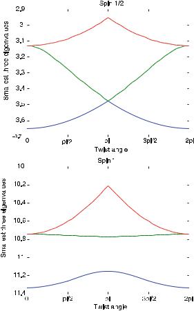
Locality Estimates for Quantum Spin Systems |
609 |
Here we have denoted by τt (·) the dynamics generated by the Hamiltonian Hθ,−θ , and P0(θ, −θ ) is the corresponding spectral projection onto the ground state. Due to the gap assumption, (76) is well-defined.
Equation (75) captures the evolution of the ground state of a doubly twisted Hamiltonian along the path θ = −θ where the effect of the first twist is canceled by the second. The trial state is obtained by using an approximation of the differential equation in (75) to describe the ground state of the singly twisted Hamiltonian Hθ,0. Introduce the parameters α > 0 and T > 0. To approximate the imaginary time evolution corresponding to an arbitrary Hamiltonian H , with dynamics τs (·), at time t > 0, we define
Aα (it, H ) = |
|
|
1 |
+∞ |
e−αs2 |
(77) |
|
|
|
−∞ τs (A) |
|
ds |
|||
|
2π i |
s − it |
|||||
for any observable A. In general, an anti-Hermitian operator of the form |
|
||||||
|
|
|
T |
|
|
|
|
Bα,T (A, H ) = − |
0 |
[Aα (it, H ) − Aα (it, H ) ]dt, |
(78) |
||||
will be used in place of (76).
Note that the observable which is evolved in (76), ∂θ Hθ,−θ , contains terms of two types. The first are localized around the twist of angle θ which correspond to
horizontal bonds (x, y) of the type x = (m, v), y = (m + 1, v), and some v VL . The second are similar, yet localized around the twist of angle −θ . We group these two types of terms together and write ∂θ Hθ,−θ = ∂1Hθ,−θ − ∂2Hθ,−θ to simplify notation. By linearity, the operator
Bα,T (∂θ Hθ,−θ , Hθ,−θ ) = Bα,T (∂1Hθ,−θ , Hθ,−θ ) − Bα,T (∂2Hθ,−θ , Hθ,−θ ). (79)
Given a sufficiently large gap γL, there is a choice of the parameters α and T for which the ground state ψ0(θ, −θ ) is well approximated by the solution of the differential equation (75) with B(θ ) replaced by Bα,T (∂θ Hθ,−θ , Hθ,−θ ). Hastings’ clever proposal is that one may also approximate the ground state of the singly twisted Hamiltonian, ψ0(θ, 0), by evolving with just the first term on the right hand side of (79) above. More concretely, consider the operator Bα,T (θ ) defined by setting Bα,T (θ ) = Bα,T (∂1Hθ,−θ , Hθ,−θ ) and solve the Hastings’ Equation given by
∂θ ψα,T (θ ) = Bα,T (θ )ψα,T (θ ) |
(80) |
with initial condition ψα,T (0) = ψ0(0, 0), i.e., the ground state of the unperturbed Hamiltonian. Under the choice of parameters α = γL/L and T = L/2, the resulting variational state ψ1 = ψα,T (2π ) may be estimated in such a way that Theorem 7 follows. We note that a particularly nice feature of the differential equation (80) is that the operator Bα,T (θ ) is anti-Hermitian, and therefore the solution remains normalized for all θ [0, 2π ]. Hastings interprets the solution of (80) as a quasiadiabatic evolution of the ground state ψ0 = ψ0(0, 0).
610 |
Bruno Nachtergaele and Robert Sims |
5.2.2 |
Locality and the Trial State |
One key technical lemma, which we use repeatedly in all of the estimates that follow, concerns the local evolution of the solution to (80). Consider a sub-volume ΛL(m) VL localized around the twist of angle θ , for example, take ΛL(m) to be
of the form [m − (L/4 − 2), m + (L/4 − 2)] × VL which is slightly less than half of
the system. Let ρα,T (θ ) and ρ0(θ, −θ ) denote the density matrices corresponding to the states ψα,T (θ ) and ψ0(θ, −θ ).
Lemma 8. Suppose there exists a constant c > 0 such that LγL ≥ c and choose α = γL/L and T = L/2. Then, there exists constants C > 0 and k > 0 such that
sup TrVL\ΛL(m)[ρα,T (θ ) − ρ0(θ, −θ )] 1 ≤ CL2ν e−kLγL .
θ [0,2π ]
Since the proof proceeds by way of contradiction, the assumption LγL ≥ c is part of the argument. Moreover, it is easy to produce a bound on γL from above that is independent of the length scale L. Lemma 8 demonstrates that if LγL is sufficiently large, then the effect of ignoring the second twist in the definition of ψα,T (θ ) is negligible when one restricts their attention to observables localized in ΛL(m). The proof of this lemma uses both the Lieb-Robinson bound, Theorem 1, and the Exponential Clustering result, Theorem 4.
5.2.3 The Estimates
The Energy Estimate: To estimate the energy of the trial state, we consider the function
E(θ ) = ψα,T (θ ), Hθ,−θ ψα,T (θ ) . |
(81) |
Due to the initial condition used to define ψα,T (θ ), we know that E(0) = E0 the ground state energy, and since H2π,−2π = HL, E(2π ) corresponds to the energy of the trial state ψ1 = ψα,T (2π ). The main idea here is to use the locality property of the trial state, i.e. Lemma 8, and the unitary equivalence of the Hamiltonians Hθ,−θ to obtain an estimate on the derivative of this function which is uniform for θ [0, 2π ]. Explicitly, we can prove the following result.
Theorem 9. Suppose there exists a constant c > 0 such that LγL ≥ c and choose α = γL/L and T = L/2. Then, there exists constants C > 0 and k > 0 such that
| ψ1, HLψ1 − E0| ≤ CL3ν−1e−kLγL .
The Orthogonality Estimate: As we mentioned before, Hastings’ quasi-adiabatic
evolution is norm preserving. In |
particular, we are guaranteed |
that ψ1 = |
ψ0 = 1. Our argument that ψ1 |
is sufficiently orthogonal to ψ0 |
makes essen- |
tial use of the fact that the total spin in each perpendicular set, VL , is half-integer. In the case of the spin-1/2, anti-ferromagnetic Heisenberg model, this corresponds to the assumption that |VL | is odd. We have the following theorem.
Locality Estimates for Quantum Spin Systems |
611 |
Theorem 10. Suppose there exists a constant c > 0 such that LγL ≥ c and choose α = γL/L and T = L/2. Then, there exists constants C > 0 and k > 0 such that
| ψ1, ψ0 | ≤ CL2ν e−kLγL .
To prove this result we observe that, although the ground state ψ0(θ, −θ ) of the perturbed Hamiltonian is not translation invariant, it is invariant with respect to “twisted” translations. In fact, let T be a unitary implementing the translation symmetry in the horizontal direction, specifically the direction in which we have imposed periodic boundary conditions, chosen such that T ψ0 = ψ0. This is possible since ψ0 is the unique ground state and the Hamiltonian is translation invariant with respect to T , i.e., T HLT = HL.
Define twisted translations by setting |
|
Tθ,θ = T Um(θ )Um+L/2(θ ) |
(82) |
where the column rotation, Un(θ ), applies the rotation eiθ Sx3 to all sites for the form x = (n, v), for some v VL . The unitary equivalence of the doubly twisted Hamiltonian Hθ,−θ to HL = H0,0 can also be expressed in terms of these column rotations
Hθ,−θ = W (θ ) H0,0W (θ ), |
(83) |
|
where |
|
|
W (θ ) = |
Un(θ ). |
(84) |
|
m<n≤m+L/2 |
|
With these definitions, it is easy to see that W (θ ) T W (θ ) = Tθ,−θ commutes with Hθ,−θ , and therefore,
Tθ,−θ ψ0(θ, −θ ) = ψ0(θ, −θ ), |
(85) |
as we claimed.
The main idea in the proof of Theorem 10 is to again use the locality properties of the solution of Hastings’ Equation (80) to show that
Tθ,0ψα,T (θ ) ψα,T (θ ). |
(86) |
Since the total spin in each VL is half-integer, again a consequence of assuming
|VL | is odd, the column rotation Um(2π ) = −1l. Clearly then, T2π,0 = −T , and therefore, T ψ1 −ψ1. As we have chosen T so that, T ψ0 = ψ0, this implies that ψ1 is nearly orthogonal to ψ0.
5.2.4 Generalizations
As we previously indicated, the proof of the multi-dimensional Lieb-Schultz-Mattis Theorem, demonstrated in [20], applies to a large variety of models. In what follows
612 |
Bruno Nachtergaele and Robert Sims |
below, we will outline a list of assumptions which define a wide class of Hamiltonians for which the LSM Theorem remains valid.
The Basic Set-Up: It is not important for our argument that the underlying sets have a lattice structure, in particular the sets VL need not be subsets of Zν . Rather, we need only assume that there is, at least, one direction of increase, which previously we labeled the horizontal direction. We make this notion concrete by assuming that there exists an increasing sequence of finite sets {VL}L≥1, exhausting some infinite set V , which are of the form VL = [1, L] × VL . We also assume a bound on the cardinality of the perpendicular sets of the form |VL | ≤ cLα for some α ≥ 0, and it is natural, but not necessary, to take α = ν − 1.
The interactions can also be of a general form. We assume that the set V is equipped with a metric d and a function F as described in Sect. 2. To start with, we work with interactions Φ Ba (V ) for some a > 0 so that the infinite volume dynamics is well defined from the beginning. In contrast to (68), the more general finite volume Hamiltonians are of the form
HL = |
Φ(X) + boundary terms, |
(87) |
X VL
where we will assume periodic boundary conditions in the horizontal direction and arbitrary boundary conditions in the other directions.
Assumption I. Our first assumption is that the interaction Φ Ba (V ) is translation invariant in the horizontal direction. This is clearly the case for the Heisenberg anti-ferromagnet, and in general, it means that for any X VL,
Φ(X + e1) = α1(Φ(X)), |
(88) |
where X + e1 is the translation of all points in X by one unit in the horizontal direction and α1(·) is the translation automorphism which maps A(n,VL ) into A(n+1,VL ) for all n Z. Here the column sets (n, VL ) are defined by (n, VL ) = {x VL : x = (n, v) for some v VL }. Due to the assumed periodicity in the horizontal direction, this translation invariance can be implemented by a unitary T AVL , i.e. Φ(X + e1) = T Φ(X)T for all X VL. This unitary T will depend on the length scale L, but we will suppress this in our notation.
Assumption II. We further assume that the interaction has a finite range R > 0 in the horizontal direction. This assumption is not strictly necessary. It is clear from the estimates in [20] that the result remains true even if the interactions are of long range with sufficiently fast decay.
Assumption III. We assume the interaction Φ has rotation invariance about one axis. Again, this is clearly the case for the Heisenberg model. In the more abstract setting, we specifically assume that for each x V there is a local hermitian matrix, which we will denote by Sx3, with eigenvalues that are either all integer or all halfinteger. These matrices are also required to be translates of one another, i.e., for any
x V , α1(Sx3) = Sx3+e1 . Rotation invariance for a general interaction Φ means that

Locality Estimates for Quantum Spin Systems |
613 |
for any X VL, |
|
|
U (θ )Φ(X)U (θ ) = Φ(X) for all θ R, |
(89) |
|
where the rotation U (θ ) is defined by |
|
|
U (θ ) = |
eiθ Sx3 . |
(90) |
|
x VL |
|
Assumption IV. We assume that the matrices introduced above, i.e. Sx3, are uniformly bounded in the sense that there exists a positive real number S for which supx V Sx3 ≤ S. In addition, we must assume an odd parity condition on the spins. Define the parity px of a site x V to be 0 if the eigenvalues of Sx3 are all integers and 1/2 if they are all half-integers. The odd parity assumption is that
p(n,v) N + 1/2, |
(91) |
v VL
for all n Z. For the spin-1/2 Heisenberg model, we satisfied this assumption by taking the cardinality of the perpendicular sets, |VL |, to be odd. In general, the sum of the spins over the perpendicular set needs to be half-integer to ensure that the column rotations Un(θ ), as defined after equation (82), satisfy Un(2π ) = −1l. As we have seen, such an identity plays a crucial role in our argument for orthogonality.
Assumption V. The ground state of HL is assumed to be non-degenerate. In this case, it is also an eigenvector of the translation T and the rotations U (θ ) introduced above. We assume that the ground state has eigenvalue one for both T and U (θ ).
Assumption VI. We assume that there are orthonormal bases of the Hilbert spaces HVL with respect to which Sx3 and Φ(X) are real for all x V and all finite X V . This assumption is satisfied by the Heisenberg model, and it is an important symmetry which allows us, in general, to prove that the ground state eigenvalue is invariant with respect to the doubly twisted Hamiltonian Hθ,−θ .
The following theorem was proven in [20].
Theorem 11. Let Φ Ba (V ) for some a > 0. If Φ satisfies assumptions I-VI above, then the gap, γL, above the ground state energy of HL satisfies
γL ≤ C |
log(L) |
(92) |
L . |
Acknowledgements R.S. would like to acknowledge the gracious hospitality provided by the Isaac Newton Institute for Mathematical Sciences where the writing of this work began. This article is based on work supported by the U.S. National Science Foundation under Grant # DMS-0605342. A portion of this work was also supported by the Austrian Science Fund (FWF) under Grant No. Y330.
614 |
Bruno Nachtergaele and Robert Sims |
References
1.I. Affleck and E. Lieb, A proof of part of Haldane’s conjecture on quantum spin chains. Lett. Math. Phys. 12, 57–69 (1986)
2.H. Araki, Gibbs states of a one dimensional quantum lattice. Commun. Math. Phys. 14, 120– 157 (1969)
3.H. Araki, K. Hepp, and D. Ruelle, Asymptotic behaviour of Wightman functions. Helv. Phys. Acta 35, 164 (1962)
4.S. Bravyi, M.B. Hastings, and F. Verstraete, Lieb-Robinson bounds and the generation of correlations and topological quantum order. Phys. Rev. Lett. 97, 050401 (2006). arXiv:quant-ph/0603121
5.J. Eisert and T.J. Osborne, General entanglement scaling laws from time evolution. Phys. Rev. Lett. 97, 150404 (2006). arXiv:quant-ph/0603114
6.K. Fredenhagen, A remark on the cluster theorem. Commun. Math. Phys. 97, 461–463 (1985)
7.R. Haag, Local Quantum Physics. Springer, Berlin (1992)
8.F.D.M. Haldane, Continuum dynamics of the 1-D Heisenberg antiferromagnet: Identification with the O(3) nonlinear sigma model. Phys. Lett. A 93, 464–468 (1983)
9.M.B. Hastings, Lieb-Schultz-Mattis in higher dimensions. Phys. Rev. B 69, 104431 (2004)
10.M.B. Hastings and T. Koma, Spectral gap and exponential decay of correlations. Commun. Math. Phys. 265, 781–804 (2006)
11.M.B. Hastings and X.-G. Wen, Quasi-adiabatic continuation of quantum states: The stability of topological ground-state degeneracy and emergent gauge invariance. Phys. Rev. B 72, 045141 (2005)
12.M. Keyl, T. Matsui, D. Schlingemann, and R. Werner, Entanglement, Haag-duality and type properties of infinite quantum spin chains. arXiv:math-ph/0604071
13.E.H. Lieb and D. Mattis, Ordering energy levels in interacting spin chains. J. Math. Phys. 3, 749–751 (1962)
14.E.H. Lieb and D.W. Robinson, The finite group velocity of quantum spin systems. Commun. Math. Phys. 28, 251–257 (1972)
15.E.H. Lieb, T. Schultz, and D. Mattis, Two soluble models of an antiferromagnetic chain. Ann. Phys. 16, 407–466 (1961)
16.T.M. Liggett, Interacting Particle Systems. Springer, Berlin (1985)
17.B. Nachtergaele, The spectral gap for some quantum spin chains with discrete symmetry breaking. Commun. Math. Phys. 175, 565–606 (1996)
18.B. Nachtergaele and R. Sims, Lieb-Robinson bounds and the exponential clustering theorem.
Commun. Math. Phys. 265, 119–130 (2006)
19.B. Nachtergaele and R. Sims, Recent progress in quantum spin systems. Markov Process. Relat. Fields 13, 315–329 (2007)
20.B. Nachtergaele and R. Sims, A multi-dimensional Lieb-Schultz-Mattis theorem. Commun. Math. Phys. 276, 437–472 (2007)
21.B. Nachtergaele, Y. Ogata, and R. Sims, Propagation of correlations in quantum lattice systems. J. Stat. Phys. 124, 1–13 (2006)
22.B. Nachtergaele, H. Raz, B. Schlein, and R. Sims, Lieb-Robinson bounds for harmonic and anharmonic lattice systems. Commun. Math. Phys. 286, 1073–1098 (2009)
23.D. Ruelle, On the asymptotic condition in quantum field theory. Helv. Phys. Acta 35, 147 (1962)
24.W. Wreszinski, Charges and symmmetries in quantum theories without locality. Fortschr. Phys. 35, 379–413 (1987)

616 |
|
|
|
|
|
|
|
|
|
|
|
|
|
Alexander Soshnikov |
||||
n |
|
≤ |
|
+ |
2/3 |
= |
|
|
= |
|
− |
∞ |
|
+ |
|
− |
2 |
|
|
2 |
xn− |
F1 |
(x) |
exp |
1/2 |
q(t ) |
(t |
x)q (t )dt |
, |
||||||||
lim P λmax |
|
|
|
|
|
|
|
|||||||||||
|
→∞ |
|
|
|
|
|
|
|
|
|
|
x |
|
|
|
|
|
(2) |
|
|
|
|
|
|
|
|
|
|
|
|
|
|
|
|
|
|
|
where q(x) is the solution of the Painléve II differential equation q (x) = xq(x) + 2q3(x) with the asymptotics at infinity q(x) Ai(x) as x → +∞. Here Ai(x) denotes the Airy function.
To consider the joint distribution of the largest eigenvalues at the edge of the spectrum, we rescale the eigenvalues as
λj(n) = 2 + ξj(n)n−2/3, j = 1, 2, . . . , n, |
(3) |
where λ(n)1 ≥ λ(n)2 · · · ≥ λ(n)n are the ordered eigenvalues of An. It then follows
from the results of [14, 19] that the random point configuration {ξj(n), 1 ≤ j ≤ n} converges in distribution on the cylinder sets to the random point process on the real line with the k-point correlation functions given by
|
ρk (x1, . . . , xk ) = det(K(xi , xj ))1≤i,j ≤k 1/2 , |
|
(4) |
|||||||||||||
where K(x, y) is a 2 × 2 matrix-valued kernel with the entries |
|
|
|
|||||||||||||
|
|
|
|
|
|
1 |
|
|
+∞ |
|
|
|
|
|
||
K11 |
(x, y) = KAiry(x, y) + |
|
Ai(x) 1 − y |
Ai(z)dz |
, |
|
(5) |
|||||||||
2 |
|
|||||||||||||||
K12 |
(x, y) = −∂y KAiry(x, y) − |
1 |
Ai(x)Ai(y), |
|
|
|
|
(6) |
||||||||
|
|
|
|
|
||||||||||||
2 |
|
|
|
|
||||||||||||
|
+∞ |
|
|
|
|
|
|
|
|
|
|
|
|
|||
K21 |
(x, y) = − x |
KAiry(z, y)dz |
|
|
+∞ |
|
|
|||||||||
|
+ |
|
1 x |
|
|
|
|
+∞ |
|
|
|
|
||||
|
|
|
|
|
Ai(z)dz + x |
Ai(z)dz |
|
Ai(z)dz |
, |
(7) |
||||||
|
2 |
|
y |
y |
||||||||||||
K22 |
(x, y) = K11(y, x), |
|
|
|
|
|
|
|
|
|
|
(8) |
||||
and the Airy kernel KAiry(x, y) is defined as |
|
|
|
|
|
|
||||||||||
|
+∞ |
Ai(x + z)Ai(y + z)dz = |
Ai(x)Ai (y) |
Ai (x)Ai(y) |
(9) |
|||||||||||
KAiry(x, y) = |
|
|
x − y |
. |
||||||||||||
|
0 |
|
|
|
|
|
|
|
|
|
|
|
− |
|
|
|
Therefore, the k-point correlation function of the limiting random point process is given by the square root of the determinant of the 2k × 2k matrix defined in (4) and (5). One can also rewrite the k-point correlation function in the pfaffian form (see e.g. [9]) which shows that the limiting random point process belongs to the family of the pfaffian random point processes (see e.g. [15]). In particular, the rightmost particle of this pfaffian random point process is given by the Tracy-Widom distribution (2). Moreover, it was shown in [12] that the asymptotic behavior of the largest eigenvalues is universal for Wigner real symmetric matrices with sub-
On Resolvent Identities in Gaussian Ensembles at the Edge of the Spectrum |
617 |
Gaussian and symmetrically distributed entries. We refer to [10] for recent results on wigner matrices with nonsymmetrically distributed entries.
Define |
|
Gn(z) = An − 2 − zn−2/3 −1 |
(10) |
for complex z with non-zero imaginary part Im z = 0. Here and throughout the
paper, we will use (An − z)−1 as the shorthand notation for the resolvent matrix
(An − zI d)−1.
Let |
|
|
|
|
|
|
|
|
|
gn,k (z) |
= |
n−2k/3 Tr Gk |
(z) |
= |
n−2k/3 Tr An |
− |
2 |
− |
zn−2/3 −k |
|
n |
|
|
|
|
||||
|
|
n |
|
|
|
|
|
|
|
|
= ξj(n) − z −k |
|
|
|
|
|
(11) |
||
|
|
1 |
|
|
|
|
|
|
|
for positive integers k = 1, 2, . . . . It can be shown that for k ≥ 2, gn,k (z) is a “local” statistic of the largest eigenvalues in the GOE. Indeed, only eigenvalues from the O(n−2/3)-neighborhood of the right edge of the spectrum give non-vanishing contribution to gn,k (z) in the limit n → ∞. For example, the joint contribution of
the eigenvalues from (−∞, 2 − δ] can be trivially bounded in absolute value by n1−2k/3|δ + zn−2/3|k = o(1) for large n uniformly in z with Re z bounded from be-
low. More delicate estimates involving the asymptotics of the one-point correlation function, imply that the joint contribution of the eigenvalues from (−∞, 2−n−2/3+ε ) to gn,k (z) is still negligible for all ε > 0 and k > 1. Moreover, the one-point correlation function ρ1(x) of the limiting pfaffian random point process defined in (3)–(9) decays super-exponentially at +∞ and grows proportionally to |x|1/2 at −∞. Consequently, if ξ = {ξj , j Z} is a random point configuration of the limiting pfaffian random process then
|
|
k |
+∞ |
k |
|
E |
|
|
|
|x − z|− ρ1(x)dx < ∞ |
(12) |
|
|ξj − z|− = |
−∞ |
|||
|
j |
|
|
|
|
for any integer k ≥ 2. The integral at the r.h.s. of (12) diverges for k = 1 which emphasizes the fact that gn,1(z) is not a “local statistic” as the main contribution to gn,1(z) = n−2/3 Tr(An − 2 − zn−2/3)−1 comes from the eigenvalues in the bulk. Moreover, it could be shown from the asymptotics of the GOE one-point correlation function that
E Tr An − 2 − zn−2/3 −1 = −n + O(n2/3). |
(13) |
Eventhough the eigenvalues from the bulk of the spectrum give the main contribution to the mathematical expectation of Tr(An − 2 − zn−2/3)−1, their joint contribution to the fluctuations of Tr(An − 2 − zn−2/3)−1 around its mean is much smaller (namely, it can be shown to be of order of constant if one smoothes their contribution by a test function with the support inside [−2 + δ, 2 − δ]). On the other hand, the largest eigenvalues of An give smaller (namely, of the order of O(n2/3)) contribution to the mean of Tr(An − 2 − zn−2/3)−1 but they give the main contribution to


620 |
Alexander Soshnikov |
eigenvalue of Mn,N are of the order of n−2. Moreover, if we consider the rescaling at the hard edge of the spectrum
(n,N ) |
|
ξ (n,N ) |
|
|
|
|
= |
|
i |
|
1 ≤ i ≤ n, |
(26) |
|
λi |
|
|
, |
|||
|
4n2 |
|||||
one can show that the random point configuration {ξi(n), 1 ≤ i ≤ n} converges in distribution on the cylinder sets to the pfaffian random point process on (0, +∞). The k-point correlation functions of the limiting process are of the same form as in (4), where K(x, y) is again a 2 × 2 matrix-valued kernel. The formulas for the entries of K(x, y) are similar to (5) with the important difference being that the Airy kernel KAiry(x, y) is replaced by the Bessel kernel
|
|
|
|
Jν (√ |
x)√ |
yJν+1(√ |
y) − Jν (√ |
y)√ |
xJν+1(√ |
|
|
|
|
|||||||||
K |
|
(x, y) |
= |
x) |
, |
(27) |
||||||||||||||||
|
|
|
|
|
|
|
|
|
|
|||||||||||||
|
Bessel |
|
|
|
|
|
|
|
2(x |
− |
y) |
|
|
|
|
|
|
|||||
|
|
|
|
|
|
|
|
|
|
|
|
|
|
|
|
|
|
|
|
|
|
|
where Jν (x) is the usual Bessel function of index ν. |
|
|
|
|
|
|
||||||||||||||||
Define |
|
|
|
|
|
|
|
|
|
|
|
|
|
t 2 −1 |
|
|
|
|
|
|
||
|
|
|
|
|
|
|
|
|
|
|
|
|
|
|
|
|
|
|
|
|||
|
|
|
|
|
|
Gn,N (t ) = |
Mn,N + |
|
, |
|
|
|
|
|
(28) |
|||||||
|
|
|
|
|
|
n2 |
|
|
|
|
|
|||||||||||
where t is a real number. Then |
|
|
|
|
|
|
|
|
|
|
|
|
|
|||||||||
|
|
|
|
|
|
|
|
|
|
|
|
|
|
|
|
|
t 2 −k |
|
||||
g |
(t ) |
|
g |
|
(t ) |
|
n−2k Tr Gk |
(t ) |
|
n−2k Tr M |
|
|
|
|
|
|
||||||
= |
|
= |
= |
n,N + n2 |
|
|||||||||||||||||
k |
|
|
n,N ,k |
|
|
|
|
n,N |
|
|
|
|
|
|
||||||||
|
|
|
n |
|
|
|
|
|
|
|
|
|
|
|
|
|
|
|
|
|
|
|
|
|
= ξi(n,N ) + t 2 −k |
|
|
|
|
|
|
|
|
|
|
|
|
(29) |
|||||||
|
|
|
|
1 |
|
|
|
|
|
|
|
|
|
|
|
|
|
|
|
|
|
|
is a “local” statistics for any positive integer k = 1, 2, 3, . . . . Indeed, one can show that the eigenvalues from the bulk of the spectrum give vanishing contribution to gk (t ). In particular, if ξ = {ξi , i N} is a random point configuration of the limiting pfaffian process, then
|
2 |
k |
|
+∞ |
|
1 |
|
|
|
E |
|
|
|
|
|
|
|
|
|
|
= |
|
|
|
t 2)k ρ1(x)dx < ∞. |
(30) |
|||
|
(ξj + t )− |
|
0 |
(x |
+ |
||||
|
j |
|
|
|
|
|
|
||
We are interested to study the joint moments of the linear statistics gk (t ), k ≥ 1. Let, as before, K = (k1, . . . , kj ), j ≥ 1, denote a multi-index, and mK stand for the corresponding joint moment
|
j |
|
|
|
mK = |
E |
kl |
. |
(31) |
|
(gl (t )) |
l=1
The following theorem holds.
Theorem 4. Let K be a non-zero multi-index, then the following equation holds:


622 |
Alexander Soshnikov |
We recall that ν = N − n ≥ 0 is the difference between the dimensions of the rectangular matrix An,N . Theorems 4 and 5 will be proved in Sect. 3.
2 Proof of Theorems 1 and 3
Let us start with the proof of Theorem 1. Our first goal is to establish (17). To this end, we consider n1/3me1 = E(n−1/3(n + Tr Gn(z))), where, as before, Gn(z) = (An − 2 − zn−2/3)−1. By using the resolvent identity
Gn(z) = An − 2 − zn−2/3 −1
|
|
= − 2 + zn−2/3 −1Id + 2 + zn−2/3 −1An An − 2 − zn−2/3 −1 |
|
|||
|
|
= − 2 + zn−2/3 −1Id + 2 + zn−2/3 −1AnGn, |
(38) |
|||
we arrive at |
|
|
|
|
|
|
n1/3me1 |
= n2/3 − 2 + zn−2/3 −1n2/3 + 2 + zn−2/3 −1n−1/3E Aij Gj i . (39) |
|||||
|
|
|
|
|
ij |
|
Here Aij |
= |
|
aij |
|
||
|
√ |
|
denote the matrix entries of An, and Gij denote the matrix entries of |
|||
|
n |
|||||
Gn(z). To calculate EAij Gj i , we recall that random variables Aij , 1 ≤ i ≤ j ≤ n, are independent. Therefore, we can first fix all matrix entries (up from the diagonal) except Aij and integrate with respect to Aij . Applying the Gaussian decoupling formula
|
Eηf (η) = σ 2Ef (η), η N (0, σ 2), |
1+δij |
(40) |
||||
with η = Aij and f (η) = Gij , and taking into account that Var(Aij ) = |
, and |
||||||
n |
|||||||
|
|
|
|
|
|
|
|
|
∂Gkl |
|
−Gki Gj l − Gkj Gil |
i = j, |
|
(41) |
|
|
∂Aij = |
|
|||||
|
−Gki Gj l |
i = j, |
|
|
|||
we arrive at |
|
|
|
|
|||
n1/3me1 = n2/3 − 2 + zn−2/3 −1n2/3 |
|
|
|
||||
|
− 2 + zn−2/3 −1n−4/3E (Gj i Gj i + Gii Gjj ). |
(42) |
|||||
|
|
|
ij |
|
|
|
|
The term n−4/3E ij Gj i Gj i |
is equal to |
|
|
|
|||
n−4/3E Gj i Gj i = En−4/3 Tr Gn2 (z) = me2 . |
|
(43) |
|||||
|
ij |
|
|
|
|
||
To deal with the term n−4/3E ij Gii Gjj , we rewrite it as

624 |
Alexander Soshnikov |
As in the case K = 0 considered above, we fix all matrix entries (up from the
diagonal) except Aij , and apply (40) with η = Aij and f (η) = Gj i (n−2/3(n +l≥2(n−2l/3 Tr Gl )kl . Taking into account (41) and the equation
∂ Tr(Gl ) |
= − |
2l(Gl+1)ij , |
(50) |
|
∂Aij |
||||
|
|
one then obtains (16) after some simple algebraic calculations. Theorem 1 is proven. The proof of Theorem 3 is quite similar. The only alteration required in the GUE
case is that one needs to replace (41) with
|
|
∂Gkl |
|
|
−Gki Gj l |
− Gkj Gil |
i = j |
(51) |
|
∂Re(Aij ) = |
|||||||
|
−Gki Gj l |
|
i = j, |
|
||||
and |
|
|
|
|
|
|
||
|
|
∂Gkl |
= −i(Gki Gj l − Gkj Gil ) |
for i = j. |
(52) |
|||
∂Im(Aij ) |
||||||||
The remaining calculations are very similar and are left to the reader.
3 Proof of Theorems 4 and 5
The proofs will be similar to the ones given in the previous section. Let us start with the proof of Theorem 4. Our first goal is to establish (33). To this end, we consider n−1me1 = E(n−3 Tr Gn,N (t )), where Gn,N (t ) was defined in (28). By using the resolvent identity
|
|
|
|
|
|
|
|
|
|
|
|
t 2 −1 |
n2 |
n2 t |
|
|
|||||
|
|
|
Gn,N = |
Mn,N + |
|
|
|
= |
|
Id − |
|
AA |
Gn,N |
(53) |
|||||||
|
|
|
n2 |
t 2 |
t 2 |
||||||||||||||||
we arrive at |
|
|
|
|
|
|
|
|
|
|
|
|
|
|
|
|
|
|
|
|
|
|
|
|
n− |
1 |
|
|
1 |
|
1 |
|
1 |
E |
|
|
|
|
|
||||
|
|
|
|
me1 |
= t 2 |
|
|
Aip Ajp Gj i . |
(54) |
||||||||||||
|
|
|
|
− n t 2 |
1≤i,j ≤n 1≤p≤N |
||||||||||||||||
|
|
|
|
|
|
|
|
|
|
|
|
|
|
|
|
|
|
|
|||
Here Aip = |
aip |
denote the matrix entries of An, and Gj i denote the matrix entries of |
|||||||||||||||||||
√ |
|
||||||||||||||||||||
n |
|||||||||||||||||||||
Gn,N (z). To calculate EAip Ajp Gj i , we again use the Gaussian decoupling formula (40) and the equation
∂Gkl |
= −Gki (At G)pl − (GA)kp Gil . |
(55) |
∂Aip |
Therefore,
On Resolvent Identities in Gaussian Ensembles at the Edge of the Spectrum |
625 |
n− |
1 |
|
|
1 |
|
|
|
1 |
|
1 |
|
E |
|
|
|
|
|
|
|
|
|
|
|
|
|
|
|
||||||||
|
me1 |
= t 2 |
+ n2 t 2 |
Ajp Gj i (GA)ip + Gii (GA)jp |
|
||||||||||||||||||||||||||||||
|
|
|
1≤i,j ≤n 1≤p≤N |
|
|||||||||||||||||||||||||||||||
|
|
|
|
|
|
|
1 |
|
1 |
|
|
|
|
|
|
|
|
|
|
|
|
|
|
|
|
|
|
||||||||
|
|
|
|
|
|
|
E |
|
|
|
|
|
|
|
|
|
|
|
|
|
|
|
|
|
|
||||||||||
|
|
|
|
− n2 t 2 |
Gii |
|
|
|
|
|
|
|
|
|
|
|
|
|
|
||||||||||||||||
|
|
|
|
|
1≤i≤n 1≤p≤N |
|
|
|
|
|
|
|
|
|
|
|
|
|
|
||||||||||||||||
|
|
|
|
|
|
|
|
|
|
|
|
|
|
|
|
|
|
|
|
|
|
|
|
|
|
|
|||||||||
|
|
|
|
1 |
|
|
|
1 |
|
1 |
|
E Tr(GAAt G) |
|
Tr(GAAt ) Tr G |
|
|
N |
|
1 |
E Tr G. |
(56) |
||||||||||||||
|
|
|
= t 2 |
+ n2 t 2 |
+ |
|
|
|
|
||||||||||||||||||||||||||
|
|
|
|
|
|
|
|
|
|
|
|
|
|
|
|
− n2 t 2 |
|
|
|
||||||||||||||||
|
|
|
|
|
|
|
|
|
|
|
|
|
|
|
|
|
2 |
|
|
|
|
|
|
|
|
|
|
|
|
|
|
|
|
|
|
Using the identity GAAt = Id − |
t |
G, the last formula can rewritten as |
|
||||||||||||||||||||||||||||||||
n2 |
|
||||||||||||||||||||||||||||||||||
|
|
|
n−1m |
|
|
|
|
1 |
|
|
|
1 |
m |
|
|
|
m |
|
|
n m |
m |
|
|
n + ν |
m |
|
, |
(57) |
|||||||
|
|
|
|
= t 2 |
|
|
|
e1 − |
|
|
2e1 − |
|
|
||||||||||||||||||||||
|
|
|
|
|
|
|
e1 |
|
+ t 2 |
|
e2 |
+ t 2 e1 − |
|
|
t 2 |
e1 |
|
|
|||||||||||||||||
which implies (33). The formula (32) can be proven along the same lines if one starts with n−1mK+e1 . Let us write
n−1mK e |
|
n−1E |
|
j |
|
|
|
|
|||
= |
|
(g1(t )) (gl (t ))kl |
|
|
|
||||||
+ 1 |
|
|
l=1 |
|
|
|
|
||||
|
|
|
|
|
|
|
|
|
|
|
|
|
|
|
|
|
|
|
|
|
|
||
|
= |
E |
n− |
3 |
|
n− |
2l |
l |
kl |
(58) |
|
|
|
|
Tr Gn,N ) |
|
Tr Gn,N |
, |
|||||
l≥1
Using the resolvent identity, we can rewrite the first term in the product as
Gn,N = n2 I d − n2 AAt Gn,N . t 2 t 2
After integration by parts and a few lines of careful calculations, we obtain (32). Theorem 5 can be proven along similar lines.
4 Non-Gaussian Case
The generalization of the Gaussian decoupling formula (40) to the non-Gaussian case can be found, for example, in [7]:
|
p |
ck |
+ |
1 |
dk f |
|
|
|
|
E |
|
|
|
E |
(ξ ) |
+ ε, |
(59) |
||
|
[ξ f (ξ )] = |
k |
! |
|
dxk |
||||
|
k=0 |
|
|
|
|
|
|
|
|
where ξ is a real random variable such that E(|ξ |p+2) < ∞, cl , l ≥ 1, are the cumulants of the random variable ξ , complex-valued function f (x) has first p + 1 continuous and bounded derivatives, and the error term satisfies the upper bound |ε| ≤
dp+1f |
(x)|E(|ξ | |
p |
+ |
2 |
) with the constant Bp+1 |
depending only on p + 1. |
Bp+1supx | dxp+1 |
|
|

626 Alexander Soshnikov
It is conjectured that the distribution of the largest eigenvalues in Wigner random matrices is universal provided the fourth moment of the matrix entries is finite. Currently, we are unable to prove this conjecture. Instead, we speculate below on the possible approach to extend the results of Theorems 1, 3–5 to the non-Gaussian
case. Let us consider a real Wigner random matrix An = |
1 |
n |
, and assume |
|
√ |
|
(aij )i,j =1 |
||
n |
||||
that the entries (aij = aj i )i<j are i.i.d. centralized random variables with the unit variance and the finite fourth moment. In addition, we assume that the diagonal entries aii , 1 ≤ i ≤ n, are i.i.d. centralized random variables, independent from the non-diagonal entries. We assume that the diagonal entries also have the finite fourth moment. Let us also assume for simplicity that Var(aii ) = 2. In an attempt to extend the result of Theorem 1 to the non-Gaussian situation, we apply the generalized decoupling formula (59). To be specific, let us concentrate our attention on
the “boundary” equation (17). Looking at (39), we apply (59) to EAij Gj i . Since
c1(aij ) = 0, c2(aij ) = 1 + δij , c3(aij ) = c3, for i < j , and Eaij4 ≤ ∞, one might wish to truncate (59) after the first three terms (i.e. p = 2) to obtain
n−1/3E Aij Gj i = −n−4/3E G2j i + Gii Gjj
ij |
ij |
|
+ n−11/6E 3Gij Gii Gjj + Gij3 + . (60) |
|
ij |
The first sum in (60) is the same as in the Gaussian case. The hope is to show that the second sum and the remainder term give negligible contributions in the limit
n → ∞. However, it is currently unclear to us how to efficiently bound the terms
n−11/6E ij Gij Gii Gjj and n−11/6E ij G3ij .
References
1.L. Arnold, On Wigner’s semicircle law for eigenvalues of random matrices. J. Math. Anal. Appl. 20, 262–268 (1967)
2.G. Ben Arous and S. Péché, Universality of local eigenvalue statistics for some sample covariance matrices. Commun. Pure Appl. Math. LVIII, 1316–1357 (2005)
3.A. Edelman, The distribution and moments of the smallest eigenvalue of a random matrix of Wishart type. Linear Algebra Appl. 159, 55–80 (1991)
4.P. Forrester, The spectrum edge of random matrix ensembles. Nucl. Phys. B 402, 709–728 (1993)
5.P. Forrester, Exact results and universal asymptotics in the Laguerre random matrix ensemble. J. Math. Phys. 35, 2539–2553 (1994)
6.J.B. Hough, M. Krishnapur, Y. Peres, and B. Virag, Determinantal processes and independence. Probab. Surv. 3, 206–229 (2006)
7.A.M. Khorunzhy, B.A. Khoruzhenko, and L.A. Pastur, Asymptotic properties of large random matrices with independent entries. J. Math. Phys. 37, 5033–5059 (1996)
8.V. Marchenko and L. Pastur, Distribution of eigenvalues of some sets of random matrices. Math. USSR Sb. 1, 457–486 (1967)
9.M.L. Mehta, Random Matrices, 3rd edn. Elsevier/Academic Press, Amsterdam (2004)
On Resolvent Identities in Gaussian Ensembles at the Edge of the Spectrum |
627 |
10.S. Péché and A. Soshnikov, Wigner random matrices with non symmetrically distributed entries. J. Stat. Phys. 129, 857–883 (2007)
11.J. Silverstein and Z. Bai, On the empirical distribution of eigenvalues of a class of largedimensional random matrices. J. Multivar. Anal. 54, 175–192 (1995)
12.A. Soshnikov, Universality at the edge of the spectrum in Wigner random matrices. Commun. Math. Phys. 207, 697–733 (1999)
13.A. Soshnikov, Determinantal random point fields. Russ. Math. Surv. 55, 923–975 (2000)
14.A. Soshnikov, A note on universality of the distribution of the largest eigenvalues in certain sample covariance matrices. J. Stat. Phys. 108, 1033–1056 (2002)
15.A. Soshnikov, Janossy densities II. Pfaffian ensembles. J. Stat. Phys. 113, 611–622 (2003)
16.C. Tracy and H. Widom, Level-spacing distribution and Airy kernel. Commun. Math. Phys. 159, 151–174 (1994)
17.C. Tracy and H. Widom, Level-spacing distribution and the Bessel kernel. Commun. Math. Phys. 161, 289–309 (1994)
18.C. Tracy and H. Widom, On orthogonal and symplectic matrix ensembles. Commun. Math. Phys. 177, 727–754 (1996)
19.C. Tracy and H. Widom, Matrix kernels for the Gaussian orthogonal and symplectic ensembles. Ann. Inst. Fourier 55, 2197–2207 (2005)
20.E. Wigner, Characteristic vectors of bordered matrices with infinite dimensions. Ann. Math. 62, 548–564 (1955)
21.E. Wigner, On the distribution of the roots of certain symmetric matrices. Ann. Math. 68, 325–328 (1958)

Energy Current Correlations for Weakly Anharmonic Lattices
Herbert Spohn
Abstract We discuss properties of the Boltzmann-Peierls equation for weakly anharmonic lattice dynamics. In particular, we explain how energy type correlations are predicted from this transport equation. An intriguing application is the famous Fermi-Pasta-Ulam β chain, for which we prove that the energy current correlations in equilibrium decay for long times as t −3/5, in the kinetic approximation.
1 Introduction
A solid transports energy. Besides the mobile electrons, one important mechanism for energy transport are the vibrations of the crystal lattice. There is no difficulty in writing down the appropriate lattice dynamics. To extract from it the thermal conductivity remains a fairly untractable problem. The most successful approach exploits that even rather close to the melting temperature the typical deviations of the crystal atoms from their equilibrium position are small as compared to the lattice constant. This observation then leads to the phonon kinetic equation, which goes back to the seminal paper by Peierls [9]. (For electron transport a corresponding idea was put forward by Nordheim [6].) Phonon kinetic theory flourished in the 50ies, an excellent account of the 1960 status being the book by Ziman [17]. Of course, transport of heat and thermal conductivity remain an important experimental research area, in particular since novel materials become available and since more extreme properties are in demand. On the other hand, if the very recent collection of articles by Tritt [15] is taken to be representative, it is obvious that after 1960 hardly any new elements have been added to the theory. The real innovation are fast and efficient molecular dynamics algorithms. The currently available techniques allow the simulation of 6 × 6 × 6 periodized lattices with two atoms per unit cell [5].
Herbert Spohn
Zentrum Mathematik and Physik Department, TU München, Boltzmannstr. 3, 85747 Garching, Germany, e-mail: spohn@ma.tum.de
V. Sidoraviciusˇ (ed.), New Trends in Mathematical Physics, |
629 |
© Springer Science + Business Media B.V. 2009 |
|


634 Herbert Spohn
In the Heisenberg picture Hx becomes time-dependent. Writing dHx (t )/dt as a divergence, the energy current can be identified with
|
1 |
|
Jx = |
4 y Zd yα(y)(−qx px+y + qx+y px ) |
(25) |
which happens to be independent of λ. To verify (25), one chooses a large box Λ with faces ∂Λ. The energy inside Λ is
|
|
HΛ(t ) = |
|
|
|
|
Hx (t ) |
(26) |
|
|
|
|
x Λ |
|
and it satisfies |
d |
|
|
|
|
HΛ(t ) = − |
nx · Jx (t ) + O (∂Λ), |
(27) |
|
|
|
|||
|
dt |
|||
|
|
x Λ |
|
|
where nx is the outward normal to Λ at x ∂Λ. The errors come from the corners of Λ and from the possibly infinite range of α.
With this input the total energy current correlation is defined by |
|
|
· Cλ(t ) = |
|
|
( · J0(t ))( · Jx (0)) β , |
(28) |
|
x Zd
where Rd , Jx Rd , “ · ” is the scalar product in Rd , and Cλ(t ) is a d × d matrix.· β refers to the thermal average with respect to Z−1e−βH . By time-stationary and time-reversal, Cλ(t ) is symmetric and it suffices to consider its numerical range. At the expense of an error of order λ, we may replace in e−βH the full Hamiltonian H by the harmonic approximation
|
|
|
|
|
|
|
|
|
|
|
|
|
|
|
|
|
|
|
|
|
|
Hha = |
Td |
dkω(k)a(k) a(k). |
|
(29) |
|||
For the total current one finds |
|
|
|
|
|
|
||||||||
|
|
|
|
|
|
|
|
|
|
|
|
|
|
|
|
|
|
|
|
1 |
|
|
|
|
|
|
|||
|
J = |
|
|
|
Td dk( ω(k))ω(k)a(k) a(k), |
|
||||||||
|
|
|
Jx = |
|
(30) |
|||||||||
|
|
|
2π |
|||||||||||
|
|
|
x Zd |
|
|
|
|
|
|
|
|
|
||
where it is used that |
|
|
|
|
|
|
|
|
x Zd · Jx can be lifted |
|||||
α = 2ω( ω). Since [Hha, J ] = 0, |
||||||||||||||
to the exponent. Thus we define the new average · β,τ |
with respect to the state |
|||||||||||||
[− |
βHha |
+ |
τ |
· |
J |
] |
. Then |
|
|
|
|
|
|
|
Z−1 exp |
|
|
|
|
|
|
|
|
|
|||||
|
|
|
· Cλ(t ) = τlim0 |
1 |
· J0(t ) β,τ + O (λ). |
(31) |
||||||||
|
|
|
|
|
||||||||||
|
|
|
|
τ |
||||||||||
|
|
|
|
|
|
|
|
|
→ |
|
|
|
|
|
The anharmonicity now resides only in the dynamics.
The limit λ → 0 on the right hand side in (31) is discussed in [13]. The initial state is spatially homogeneous and determines the Wigner function Wβ,τ (k) through
Energy Current Correlations for Weakly Anharmonic Lattices |
|
|
|
635 |
||
a(k ) a(k) β,τ |
= δ(k − k )Wβ,τ (k) |
|
|
(32) |
||
with |
|
− τ ( · ω(k))ω(k) |
|
− 1 |
|
|
Wβ,τ (k) = |
exp βω(k) |
|
−1. |
(33) |
||
On the kinetic time scale, λ−2t , the Wigner function Wβ,τ |
evolves to Wτ (t ) which |
|||||
is determined as the solution of the spatially homogeneous Boltzmann equation. For our model, i.e. for the anharmonic on-site potential V3, it reads
|
|
|
|
|
|
|
|
|
|
|
|
|
|
|
∂ |
|
|
|
|
|
|
|
|
|
|
|
|
|
|
|
|
|
|
|
|
|
|
|
|
|
|||
|
|
|
|
|
|
|
|
|
|
|
|
|
|
|
|
W (t ) = C (W (t )) |
|
|
|
|
|
|
|
|
|
|
|
|
(34) |
||||||||||||||
|
|
|
|
|
|
|
|
|
|
|
|
|
|
∂t |
|
|
|
|
|
|
|
|
|
|
|
|
|||||||||||||||||
with the collision operator |
|
|
|
|
|
|
|
|
|
|
|
|
|
|
|
|
|
|
|
|
|
|
|
|
|
|
|
|
|
|
|
|
|
|
|
||||||||
|
π |
|
|
|
|
|
|
|
|
|
|
|
|
|
|
|
|
|
|
|
|
|
|
|
|
|
|
|
|
|
|
|
|
|
|
|
|
|
|
|
|||
C (W )1 = |
|
T2d dk2dk3(ω1ω2ω3)−1 |
|
|
|
|
|
|
|
|
|
|
|
|
|
|
|
|
|
|
|
|
|
|
|||||||||||||||||||
2 |
|
|
|
2 |
− |
3 |
|
˜ 1 |
|
˜ 2 |
|
3 |
− |
|
1 |
2 |
|
˜ 3 |
|
|
|
||||||||||||||||||||||
× { |
2δ(ω |
1 + |
|
ω |
2 |
|
− |
|
|
3 |
)δ(k |
1 + |
k |
|
|
W |
|
|
) |
|
|
||||||||||||||||||||||
+ |
|
|
|
|
|
|
|
|
|
ω |
|
|
|
|
|
|
k |
)(W |
W |
|
|
W |
W |
W |
|
|
|||||||||||||||||
δ(ω |
1 − |
ω |
2 − |
ω |
3 |
)δ(k |
1 − |
k |
2 − |
3 |
|
˜ 1 |
|
2 |
W |
3 − |
|
1 |
˜ |
2 ˜ |
3 |
} |
|
(35) |
|||||||||||||||||||
|
|
|
|
|
|
|
|
|
|
|
|
|
|
|
|
|
k )(W |
W |
|
|
W |
W W |
) . |
||||||||||||||||||||
Here we use the shorthands W |
j |
|
|
= |
W (k |
), ω |
j = ω(kj ), j |
|
|
|
|
|
|
|
W (k) |
= |
|||||||||||||||||||||||||||
1 + W (k). Using (30), the |
|
|
|
|
|
|
|
|
j |
|
|
|
|
= 1, 2, 3, and |
˜ |
|
|||||||||||||||||||||||||||
average in (31) becomes then |
|
|
|
|
|
|
|
|
|
|
|
|
|||||||||||||||||||||||||||||||
|
|
|
1 |
|
|
|
|
|
|
|
|
|
|
|
|
|
|
|
|
|
|
|
|
|
|
|
|
|
|
|
|
|
|||||||||||
· J0(λ−2t ) β,τ |
|
= |
|
|
|
|
dk( · ω(k))ω(k)Wτ (k, t ) + O (λ). |
|
(36) |
||||||||||||||||||||||||||||||||||
|
2π |
|
Td |
|
|||||||||||||||||||||||||||||||||||||||
The next task is to take the limit τ → 0 in (31). One has Wβ,0(k) = (eβω(k) − 1)−1
which is a stationary solution of (34). Thus the limit τ |
→ 0 amounts to linearize |
||||||||||||||
(35) at the equilibrium Wigner function |
|
|
|
|
|
|
|
|
|||||||
|
|
|
|
Wβ (k) = (eβω(k) − 1)−1, |
|
|
(37) |
||||||||
to say |
|
|
|
|
|
|
|
|
|
|
|
|
|
(τ 2). |
|
|
W |
|
= |
W |
β + |
τ W |
|
W |
( |
· |
ω)ω |
+ O |
(38) |
||
|
|
β,τ |
|
|
β |
˜ β |
|
|
|
|
|||||
Note that |
dk( ω)ωWβ |
= 0. As suggested by (38), with a significance which |
|||||||||||||
will become more convincing in the context of the Gaussian fluctuation theory, see Sect. 5, the natural linearization of C is
|
|
|
|
C |
(W |
β |
+ |
|
|
β |
˜ β |
f ) |
= − |
δLf |
+ O |
(δ2). |
|
|
|
|
|
|
|
|
|
|
(39) |
|||||||||||
|
|
|
|
|
|
|
|
|
δW |
W |
|
|
|
|
|
|
|
|
|
|
|
|
|
|
|
|
||||||||||||
From (35) one deduces |
|
|
|
|
|
|
|
|
|
|
|
|
|
|
|
|
|
|
|
|
|
|
|
|
|
|
|
|
|
|
|
|
|
|||||
|
π |
|
|
|
|
|
|
|
|
|
|
|
|
|
|
|
|
|
|
|
|
|
|
|
|
|
|
|
|
|
|
|
|
|
|
|
||
(Lf )1 = |
|
|
T2d dk2dk3(ω1ω2ω3)−1 |
|
|
|
|
|
|
|
|
|
|
|
|
|
|
|
|
|
|
|
|
|
|
|||||||||||||
2 |
|
|
2 − |
3 |
|
˜ |
β1 |
|
˜ |
β2 |
|
β3 |
|
1 |
+ |
|
|
2 |
− |
3 |
|
|||||||||||||||||
|
× |
(2δ(ω |
1 |
+ |
ω |
2 |
− |
3 |
)δ(k |
1 + |
k |
|
|
W |
(f |
f |
) |
|||||||||||||||||||||
|
|
|
|
|
|
|
|
ω |
|
|
|
|
k |
)W |
|
W |
|
|
|
|
|
|
|
f |
||||||||||||||
|
+ |
δ(ω |
1 − |
ω |
2 |
|
|
|
|
|
|
|
|
|
|
|
|
W |
β1 |
W |
β2 |
W |
β3 |
(f |
1 − |
f |
2 |
− |
f |
)). |
||||||||
|
|
|
− ω3)δ(k1 − k2 − k3) ˜ |
|
|
|
|
3 |
|
(40) |
||||||||||||||||||||||||||||
|
|
|
|
|
|
|
|
|
|
|
|
|
|
|
|
|
|
|
|
|
|
|
|
|
|
|
|
|
|
|
|
|
|
|
|
|
|
|

Energy Current Correlations for Weakly Anharmonic Lattices |
637 |
4 The Linearized Collision Operator
If one accepts the argument leading to (42), the remaining task is to study the spectral properties of the linearized collision operator, from which the time decay of Ckin(t ) can be inferred. While this looks like a conventional mathematical physics problem, the difficulty comes from the energy-momentum constraint. Only in a few special cases there is an explicit solution. Otherwise one has to work with the implicit definition. In fact, there can be no solution at all, in which case L = 0, or several solutions, in which case one has to sum over all collision branches.
(i) quadratic form. For three phonon processes, on-site potential V3, the quadratic form of the linearized collision operator L = L3 is given by
|
g, L3f |
= |
π |
|
|
|
|
dk1dk2dk3(ω1ω2ω3)−1δ(ω1 |
+ |
ω2 |
− |
ω3)δ(k1 |
+ |
k2 |
− |
k3) |
|||||||||||||||||||||||||||||||||||||||||||
|
|
|
|
|
|
|
|||||||||||||||||||||||||||||||||||||||||||||||||||||
2 T3d |
|||||||||||||||||||||||||||||||||||||||||||||||||||||||||||
|
|
|
|
|
|
|
|
|
|
|
|
|
|
|
|
|
|
|
|
|
|
|
|
|
|
|
|
|
|
|
|
|
|
|
|
|
|
|
|||||||||||||||||||||
|
|
|
× |
W |
|
|
|
|
|
|
|
W |
(g |
1 + |
g |
2 |
− |
g |
3 |
)(f |
1 + |
f |
2 − |
f |
|
). |
|
|
|
|
|
|
|
|
|
|
|
|
|
(48) |
|||||||||||||||||||
|
|
|
|
|
β1Wβ2 |
˜ β3 |
|
|
|
|
|
|
|
|
|
|
|
|
|
3 |
|
|
|
|
|
|
|
|
|
|
|
|
|
|
|
||||||||||||||||||||||||
Correspondingly for the on-site potential V4 one has |
|
|
|
|
|
|
|
|
|
|
|
|
|
|
|
|
|
|
|
|
|
|
|
|
|
||||||||||||||||||||||||||||||||||
g, L4f = |
3π |
· |
|
3 |
|
dk1dk2dk3dk4(ω1ω2ω3ω4)−1 |
|
|
|
|
|
|
|
|
|
|
|
|
|
|
|
|
|
|
|
|
|
||||||||||||||||||||||||||||||||
4 |
|
4 |
|
|
|
|
|
|
|
|
|
|
|
|
|
|
|
|
|
|
|
|
|
|
|
|
|||||||||||||||||||||||||||||||||
|
|
|
× δ(ω1 + ω2 − ω3 − ω4)δ(k1 + k2 − k3 − k4) |
|
|
2 |
− |
|
|
3 − |
|
4 |
|
|
|||||||||||||||||||||||||||||||||||||||||||||
|
|
|
× |
W |
β1 |
W |
β2 ˜ β3 |
˜ β4 |
(g |
1 |
+ |
g |
2 − |
g |
3 |
− |
|
|
4 |
)(f |
1 |
+ |
f |
|
f |
|
) |
||||||||||||||||||||||||||||||||
|
|
|
|
|
|
|
|
|
|
|
|
W |
W |
|
|
|
|
|
|
|
|
|
|
|
|
g |
|
|
|
|
|
|
|
|
|
|
f |
||||||||||||||||||||||
|
|
|
|
|
|
3π |
|
|
|
|
|
|
|
|
|
|
|
|
|
|
|
|
|
|
|
|
|
|
|
|
|
|
|
|
|
|
|
|
|
|
|
|
|
|
|
|
|
|
|
|
|
|
|
|
|||||
|
|
|
+ |
|
|
|
|
dk1dk2dk3dk4(ω1ω2ω3ω4)−1δ(ω1 + ω2 |
+ ω3 − ω4) |
||||||||||||||||||||||||||||||||||||||||||||||||||
|
|
|
|
|
|
|
|
|
|||||||||||||||||||||||||||||||||||||||||||||||||||
|
|
|
4 |
|
|
|
+ |
||||||||||||||||||||||||||||||||||||||||||||||||||||
|
|
|
× |
δ(k |
1 |
k |
2 + |
k |
3 − |
|
4 |
)W |
β1 |
W |
β2 |
W |
β3 |
|
|
˜ β4 |
(g |
1 + |
g |
2 |
+ |
g |
3 − |
|
4 |
) |
|||||||||||||||||||||||||||||
|
|
|
|
|
|
|
|
|
|
|
|
|
k |
|
|
|
|
|
|
|
W |
|
|
|
|
|
|
|
|
|
|
g |
|
||||||||||||||||||||||||||
|
|
|
× (f1 + f2 + f3 − f4) |
|
|
|
|
|
|
|
|
|
|
|
|
|
|
|
|
|
|
|
|
|
|
|
|
|
|
|
|
|
|
|
|
|
|
|
|
||||||||||||||||||||
|
|
= f, L4pf + f, L4tf . |
|
|
|
|
|
|
|
|
|
|
|
|
|
|
|
|
|
|
|
|
|
|
|
|
|
|
|
|
|
|
|
|
|
|
|
|
(49) |
||||||||||||||||||||
L4p corresponds to the collision of a pair of phonons and L4t to a merger of three phonons into a single one, and its time reversal. The quadratic forms for L3, L4p, L4t (for notational simplicity from now on commonly denoted by L) are somewhat formal. Firstly, if ω(0) = 0 and ω(k) > 0 otherwise, the smooth functions g, f have to vanish at k = 0. More seriously, the proper definition of the δ-function requires to study more carefully the solutions to the energy constraint
ω(k1) + ω(k2) = ω(k1 + k2), |
(50) |
say in the case of L3. For the purpose of our exposition, let us simply assume that the quadratic form defines L as a self-adjoint operator. Clearly, L ≥ 0 sincef, Lf ≥ 0. As ( · ω)ω is bounded, one has
· Ckin(t ) ≤ (2π )−2 ( · ω)ω, ( · ω)ω . |
(51) |
638 Herbert Spohn
(ii) zero subspace. To establish that limt →∞ Ckin(t ) = 0, ( · ω)ω has to be orthogonal to the zero subspace of L. There seems to be no cheap argument and one
has to study the solutions to |
|
Lf = 0. |
(52) |
From (48), (49) it follows that f has to be a collisional invariant, see [13, 14] for the definition. Considering only the first summand of (49), there is a general argument [14], that the solutions to f, L4pf = 0 are spanned by 1, ω. Note that1, ( · ω)ω = 0, ω, ( · ω)ω = 0. The constant function results from phonon number conservation in a pair collision. This conservation law will be destroyed by adding a little bit of either three-phonon, L3, or the second term of the four-phonon processes, L4t. The zero subspace is then one-dimensional and spanned by ω only. For L3 of (48), the classification of the collisional invariants is an open problem.
(iii) spectral gap. If L has a spectral gap, the energy current correlation decays exponentially. If in addition ( · ω)ω is orthogonal to the zero subspace of L, then the conductivity, as the time-integral over Ckin(t ), is finite (and non-zero). In
particular (46) holds. |
|
|
|
|
|
|
|
|
|
|
|
|
|
|
|
|
|
|
|
|
|
|
|
|
|
|
|
|
|||
L is a sum of a multiplication operator and an integral operator, |
|
|
|
||||||||||||||||||||||||||||
|
|
|
|
|
|
|
|
|
|
|
|
|
|
|
|
|
|
|
|
|
|
|
|
|
|
|
|
|
|
|
|
L = V + I, |
|
Vf (k) = V (k)f (k), |
|
|
If (k) = |
|
|
Td |
dk I (k, k )f (k ), |
(53) |
|||||||||||||||||||||
where, say in the case of L3, |
|
|
|
|
|
|
|
|
|
|
|
|
|
|
|
|
|
|
|
|
|
|
|
|
|
|
|||||
|
|
|
|
|
|
|
|
|
|
|
|
|
|
|
|
|
|
|
|
|
|
|
|
|
|
|
|
|
|
|
|
|
|
π |
|
|
|
|
|
|
|
|
|
|
|
|
|
|
|
|
|
|
|
|
|
|
|
|
|
|
|
||
|
= |
|
(k)ω(k)−1 |
|
|
|
|
|
|
|
|
|
|
|
+ |
|
|
|
) −1 |
|
|
|
|
||||||||
V (k) |
|
W |
|
|
dk |
|
ω(k |
)ω(k |
k |
|
|
|
|
|
|||||||||||||||||
|
|
|
|
|
|
|
|
|
|||||||||||||||||||||||
|
2 β |
|
|
|
Td |
|
|
1 |
|
|
1 |
|
|
|
|
1 |
|
|
|
|
|
|
|
||||||||
|
|
× |
2δ(ω(k) |
+ |
ω(k |
) |
− |
ω(k |
+ |
k |
))W |
|
|
(k |
)W |
(k |
+ |
k1) |
|
||||||||||||
|
|
|
|
|
|
1 |
|
|
|
1 |
|
|
|
β |
|
|
1 |
|
˜ β |
|
|
(54) |
|||||||||
|
|
+ δ(ω(k) − ω(k1 |
) |
− |
ω(k |
+ |
k |
|
))W |
β |
(k |
)W |
(k |
+ |
k |
) . |
|||||||||||||||
|
|
|
|
|
|
1 |
|
˜ |
|
|
|
1 |
|
˜ β |
|
1 |
|
|
|||||||||||||
The integral kernel I (k, k ) is implicitly defined. It has no definite sign and tends to be divergent on lower-dimensional submanifolds of Td × Td . It would be useful to know under what conditions the integral operator I is compact.
In the very common relaxation time approximation, I is simply dropped and one
sets in approximation |
|
|
|
|
|
|
|
|
|
|
|
|
|
|
|
||||
|
· |
C |
kin |
(t ) |
= |
(2π )−2 |
|
( |
· |
ω)ω, e−|t |/τ W |
β |
W |
β |
( |
· |
ω)ω |
|
(55) |
|
|
|
|
|
|
|
|
˜ |
|
|
|
|||||||||
with the relaxation time |
|
|
|
|
|
|
|
|
|
|
|
|
|
|
|
||||
|
|
|
|
|
|
τ (k) |
= |
|
|
|
˜ |
|
|
|
|
|
|
|
(56) |
|
|
|
|
|
|
|
Wβ (k)Wβ (k)V (k)−1, |
|
|
|
|
|
|
||||||
see (44).
(iv) FPU chains. The Fermi-Pasta-Ulam chain is the special case d = 1 with nearest neighbor coupling and no quantization. For a harmonic on-site potential the dispersion relation is ω(k) = (ω02 + 1 − cos(2π k))1/2, k T. Although d = 1, the conservation laws of energy and momentum allow for non-degenerate pair collision

Energy Current Correlations for Weakly Anharmonic Lattices |
639 |
and L4p = 0, while L4t = 0 [10, 1, 4]. There are fairly explicit formuli for the potential V and the integral kernel I [3]. For ω0 > 0 and a quartic on-site potential V4, the linearized collision operator has a gap and the zero subspace is two-dimensional. The gap seems to close as ω0 → 0. On the basis of numerical simulations, the conductivity should be finite even for ω0 = 0 [1]. The FPU-β chain has the nonlinearity
Vdi4. V and I has been computed by Pereverzev [10]. He uses the relaxation time
−3/5
approximation and finds that Ckin(t ) = t for large t . Using a resolvent expansion, in [4] we prove corresponding sharp bounds and thereby confirm the relaxation time approximation in this particular case. For a finite chain of length N with thermal reservoirs at both ends, the energy transport is then anomalous and the thermal conductivity diverges as N 2/5, which seems to be in agreement with molecular dynamics. For a more detailed discussion we refer to [2], Sect. 6.
5 Gaussian Fluctuation Theory
Energy transport can be viewed in the more general context of time-dependent Gaussian fluctuation theory close to thermal equilibrium. For low density gases this link is reviewed in [11] with further examples discussed in [12]. The purpose of this section is to explain how phonon kinetic theory makes no exception. In [11, 12] spatial variation is included. Since our exposition deals only with the spatially homogeneous system, we stick to such a set-up also for the fluctuation theory.
Physically, one considers time-dependent fluctuations in equilibrium for the number of phonons with wave number k. Technically one has to sum over phonons in a small volume element in k-space. To be more precise we partition the tours T = [−1/2, 1/2] by a grid with spacing ε and denote it by Tε . (Tε )d corresponds to the crystal volume [1, . . . , l]d Zd with periodic boundary conditions, l = 1/ε. Let f : Td → R be a smooth test function. Then the fluctuation field, indexed by f and t , is defined through
ξ ε (f, t ) = εd/2 |
|
. |
|
f (k) aε (k, t ) aε (k, t ) − aε (k) aε (k) β |
(57) |
k (Tε )d
aε (k, t ) depends on ε through the finite crystal volume ε−d , through setting λ2 = ε, and through the rescaled time ε−1t in microscopic units. The claim is that, in distribution, the limit
lim ξ ε (f, t ) |
= |
ξ |
(f ) |
(58) |
ε 0 |
t |
|
|
|
→ |
|
|
|
|
exists and that the limit random field ξt (f ) is classical. In fact, the limit field should be jointly Gaussian and governed by the linear Langevin equation
∂ |
|
∂t ξt (k) = Aξt (k) + Bηt (k), |
(59) |
640 |
Herbert Spohn |
where ξt (f ) = Td dkf (k)ξt (k). A is the generator from the linearized Boltzmann equation, compare with (41), and ηt is normalized Gaussian white noise with
E(ηt (k)ηt (k )) = δ(t − t )δ(k − k ). |
(60) |
The linear operator B controls the strength and correlations for the noise input to the various k-modes.
The main observation of the fluctuation theory is the relationship between A and B through the equal-time equilibrium fluctuations. We set, as a linear operator,
|
|
g, Cf |
|
|
lim |
ε |
(g, 0)ξ |
ε |
(f, 0) β . |
|
(61) |
||||||||||
|
|
|
|
|
= ε |
0 ξ |
|
|
|
|
|||||||||||
|
|
|
|
|
|
|
→ |
|
|
|
|
|
|
|
|
|
|
|
|
|
|
Using that |
|
|
|
|
|
|
− |
|
|
|
|
|
|
|
|
|
|
|
|
||
|
|
|
|
|
|
|
|
|
|
|
|
|
|
(62) |
|||||||
a (k1)a(k2)a |
(k3)a(k4) |
β |
|
|
a (k1)a(k2) β |
|
a(k3) a(k4) |
β |
|||||||||||||
δ(k |
1 − k4)δ(k2 |
|
|
|
|
|
W |
|
(k |
), |
|
|
|
|
|
|
|
|
|
||
|
− k3)Wβ (k1) ˜ |
β |
2 |
|
|
|
|
|
|
|
|
|
|
||||||||
one obtains |
|
|
|
|
|
|
|
|
|
|
|
|
|
|
|
|
|
|
|
|
|
|
|
g, Cf |
= |
|
|
|
|
|
|
|
W |
|
(k)f (k), |
(63) |
|||||||
|
|
|
Td |
dkg(k)Wβ (k) |
˜ β |
|
|
|
|
|
|
||||||||||
in other words C is the operator of multiplication by |
|
|
W |
β |
. The fluctuation-dissi- |
||||||||||||||||
Wβ |
˜ |
|
|
||||||||||||||||||
pation relation takes then the form |
|
|
|
|
|
|
|
|
|
|
|
|
|
|
|
||||||
|
|
|
|
AC + CA = −BB . |
|
|
|
|
|
|
(64) |
||||||||||
Since AC = L = L = CA , one concludes that the noise strength is |
|
||||||||||||||||||||
|
|
|
|
|
|
BB = 2L. |
|
|
|
|
|
|
|
|
(65) |
||||||
A posteriori this identity explains also the at first sight unexpected linearization in (39). Only then the linearized operator is symmetric, as is obvious from (65).
Solving (59), the covariance of the stationary fluctuation field is given by
|
ξt (g)ξ0 |
= |
|
(66) |
|
(f ) |
g, eA|t |Cf , |
in agreement with the special case f = g = (2π )−1( · ω)ω of interest in Sect. 4.
Acknowledgements I am deeply grateful to Jani Lukkarinen for continuing discussions on weakly nonlinear wave equations.
References
1.K. Aoki, J. Lukkarinen, and H. Spohn, Energy transport in weakly anharmonic chains. J. Stat. Phys. 124, 1105–1129 (2006)
Energy Current Correlations for Weakly Anharmonic Lattices |
641 |
2.S. Lepri, R. Livi, and A. Politi, Thermal conductivity in classical low-dimensional lattices. Phys. Rep. 377, 1–80 (2003)
3.J. Lukkarinen, unpublished notes
4.J. Lukkarinen and H. Spohn, Anomalous energy transport in the FPU-β chain. Commun. Pure Appl. Math. 61, 1753–1786 (2008)
5.A.J.H. McGaughey and M. Kaviany, Thermal conductivity decomposition and analysis using molecular dynamics simulations, Part I. Lennard-Jones argon. Int. J. Heat Mass Transfer 47, 1783–1798 (2004)
6.L.W. Nordheim, On the kinetic method in the new statistics and its application in the electron theory of conductivity. Proc. R. Soc. 119, 689–698 (1928)
7.M. Omini and A. Sparavigna, An iterative approach to the phonon Boltzmann equation in the theory of thermal conductivity. Physica B 212, 101–112 (1995)
8.M. Omini and A. Sparavigna, Beyond the isotropic-model approximation in the theory of thermal conductivity. Phys. Rev. 53, 9064–9073 (1996)
9.R.E. Peierls, Zur kinetischen Theorie der Wärmeleitung in Kristallen. Ann. Phys. 3, 1055– 1101 (1929)
10.A. Pereverzev, Fermi-Pasta-Ulam-β lattice: Peierls equation and anomalous heat conductivity. Phys. Rev. E 68, 056124 (2003)
11.H. Spohn, Fluctuation theory for the Boltzmann equation. In: Montroll, E.W., Lebowitz, J.L. (eds.) Studies in Statistical Mechanics X, pp. 225–251. North-Holland, Amsterdam (1983)
12.H. Spohn, Large Scale Dynamics of Interacting Particles. Texts and Monographs in Physics. Springer, Heidelberg (1991)
13.H. Spohn, The phonon Boltzmann equation, properties and link to weakly anharmonic lattice dynamics. J. Stat. Phys. 124, 1041–1104 (2006)
14.H. Spohn, Collisional invariants for the phonon Boltzmann equation. J. Stat. Phys. 124, 1131– 1135 (2006)
15.T.M. Tritt, Thermal Conductivity, Theory, Properties, Applications. Physics of Solids and Liquids. Springer, Berlin (2005)
16.C.B. Walker, X-ray study of lattice vibrations in aluminium. Phys. Rev. 103, 547–557 (1956)
17.J.M. Ziman, Electrons and Phonons. Springer, Berlin (1962)


644 Charles M.Newman and Daniel L. Stein
H = − |
Jxy σx σy − h σx , |
(1) |
<x,y> |
x |
|
where x is a site in Zd , σx = ±1 is the spin at site x, the spin couplings Jxy are independent, identically distributed random variables, h is an external magnetic field, and the first sum is over nearest neighbor pairs of sites only. We will choose h = 0 and the Jxy to be taken from the standard normal distribution N (0, 1); consequently, (1) has global spin inversion symmetry.
A pure phase α of an EA spin glass (at a sufficiently low temperature T in a sufficiently high dimension d) should then be characterized by a vanishing magne-
tization per spin |
|
|
|
|
1 |
|
|
|
|
M α = Llim |
|
|
|
|
|
σx α |
(2) |
||
|
|
|
|
|
|
||||
|
| |
Λ |
L| |
||||||
→∞ |
|
|
x ΛL |
|
|||||
accompanied by a nonvanishing “EA order parameter,” |
|
||||||||
qEA = Llim |
|
|
|
1 |
|
|
σx α2 , |
(3) |
|
|
|
|
|
|
|||||
| |
Λ |
|
|
|
|||||
→∞ |
|
|
|
L| x ΛL |
|
||||
where ΛL is a cube of side length L and volume |ΛL| centered at the origin, and· α denotes a thermal average in the pure state α. It is generally assumed that qEA, which depends on d and T , is independent of α.
2The Sherrington-Kirkpatrick Model and the Parisi Replica Symmetry Breaking Solution
The Sherrington-Kirkpatrick (SK) model [35] is an infinite-range version of the EA model in which mean field theory is presumably exact. For a system of N spins in zero field the SK Hamiltonian is
√ |
|
|
HN = −(1/ N ) |
Jij σi σj , |
(4) |
1≤i<j ≤N
where the couplings Jij are again i.i.d. N (0, 1) r.v.’s. This model has a sharp phase transition at Tc = 1 [35] (see also [7, 39]).
The low-temperature phase has an unusual thermodynamic structure, worked out by Parisi and collaborators in a series of papers [33, 34, 10, 11]. Following the procedures underlying the analysis, it came to be known as replica symmetry breaking (RSB). The main features of this structure include an infinity of pure thermodynamic states [34] with the features of non-self-averaging and ultrametricity of spin overlap functions [10, 11]. For details see [3, 4, 12, 36, 5]. A number of features (though not all) of the Parisi solution for the SK model have been rigorously verified; see, for example [2, 7, 37–39]. Many workers in the field now believe that
Title Suppressed Due to Excessive Length |
645 |
the essential physical features of the low-temperature phase of the SK model are understood.
3 Open Problems
For the more realistic EA model, the nature of the low-temperature phase, or even the existence of such a phase, remains open, even from a nonrigorous physics standpoint. Some of the basic open questions are:
Does the EA Ising model really have an equilibrium phase transition above some lower critical dimension dc ?
If the answer to the above question is yes, is the spin-flip symmetry broken in the low-temperature phase (i.e., is qEA > 0)?
If the answer to both of the above questions is yes, what is the number of equilibrium pure state pairs for 0 < T < Tc (d) and ground state pairs (at T = 0)?
If there exist infinitely many equilibrium pure states in some dimensions and at some temperatures, are they organized according to the mean-field RSB picture (i.e., nontrivial mixtures of pure states with non-self-averaging and ultrametricity of overlaps)?
We have argued [18, 19, 28, 29] that the proper mathematical tool to address these last two questions (which we hereafter focus on) is the metastate.
4 Metastates
Consider an EA spin glass with fixed coupling realization, hereafter denoted J . If there exist many pure states, a sequence of volumes ΛL with boundary conditions chosen independently of the couplings will generally not converge to a limiting thermodynamic state, in the sense that correlations σi1 · · · σin L, computed in ΛL from the finite-volume Gibbs state (with, e.g., periodic boundary conditions), will not have a single limit as L → ∞ but rather many different limits along different subsequences of L’s (necessarily chosen in a J -dependent manner). We have called this phenomenon chaotic size dependence [14]. Such behavior in L is analogous to chaotic behavior in time t along the orbit of a dynamical system: the behavior of any particular orbit is deterministic but effectively unpredictable, appearing to be a random sample from some distribution κ on the state space of the dynamical system. Nevertheless, one can in principle reconstruct κ by keeping a record of the proportion of time the particle spends in each coarse-grained region of state space. Similarly, one can prove [18, 19] that for inhomogeneous (disordered) systems like spin glasses, a similar distribution exists: roughly speaking, the fraction of ΛL’s in which a given thermodynamic state Γ appears converges. The state Γ can be either pure or mixed, depending on the boundary conditions.
646 |
Charles M.Newman and Daniel L. Stein |
Mathematically, a metastate κ is a probability measure on the space of all (fixed J ) thermodynamic states. Of course, the metastate depends on the boundary conditions used: we will refer to the metastate constructed from a deterministic sequence of volumes, all with periodic boundary conditions, as the “periodic b.c. metastate”, and similarly for the antiperiodic b.c. metastate, the free b.c. metastate, and so on. One can also construct metastates in which the b.c.’s vary with L.
A simplified empirical construction of κ would be as follows: consider a “micro-
canonical” ensemble κL, in which each of the finite volume Gibbs states ρ(1), . . . , ρ(L) in volumes Λ1, . . . , ΛL has weight L−1. Then κ = limL→∞ κL. The meaning of the limit is that for every well-behaved function g(·) on states,
|
|
|
L |
|
|
|
|
|
|
lim L−1 |
|
|
g(ρ( )) |
= { |
g(Γ ) |
}κ |
, |
(5) |
|
L |
→∞ |
|
= |
1 |
|
|
|
||
|
|
|
|
|
|
||||
|
|
|
|
|
|
|
|
|
|
where the bracket {.}κ denotes the average over the metastate κ.
There is an alternative (and earlier) construction due to Aizenman and Wehr [1], where one replaces the microcanonical ensemble κL by the ensemble of states obtained by varying the couplings outside ΛL. Here, for every well-behaved function F of finitely many couplings and finitely many correlations,
Llim [F (J , ρ(L))]av = {F (J , Γ )}κ(J ) av , |
(6) |
→∞ |
|
where [.]av denotes the average over the quenched coupling distribution. It has not been proved that these relatively simple limits, using all ’s and L’s, exist, but it can be proved [19] that there exist deterministic (i.e., J -independent) subsequences of’s and L’s for which limits such as in both (5) and (6) exist and yield the same κ(J ). (In some cases these subsequences may need to be sparse; see, e.g., [8, 9].)
5 Invariance and Ergodicity
The metastate is a central tool we will use to analyze whether the type of ordering present in the RSB solution of the SK model can hold in more realistic short-ranged models. We will combine it with some basic invariance and ergodicity properties of functions on the disorder random variables to draw rigorous conclusions about some of these functions that are of physical and mathematical interest.
Our results basically apply to any disorder distribution ν(J ) in which the couplings are independent, identically distributed random variables (although parts of the arguments are most easily carried out when each coupling has a continuous distribution as in the Gaussian case). At some fixed dimension d and temperature T , consider a function F (d, T , J ) on Zd that is translation-invariant on the couplings in at least one coordinate. For example, F (d, T , J ) might denote the number of pure states, or the spin overlap function [12] or the sum of the squares of the pure state weights (if there are a countable number of pure states) averaged over the
Title Suppressed Due to Excessive Length |
647 |
metastate. Then it can be proved that F (d, T , J ) is constant in J almost surely; i.e., it is the same for a.e. J , at fixed T and d. Of course, F (d, T , J ) can have some dependence on both d and T . It also can depend on ν, although that dependence is not explicitly indicated. But once all of these are determined, it cannot depend on any realization J of the couplings (outside of a set of measure zero). In the language of spin glass theory, F is a self-averaged quantity.
The proof of such a statement lies in a straightforward use of the ergodic theorem [13], and depends on three ingredients: measurability of F as a function of J , translation-invariance of F with respect to a uniform shift of the xy indices of the couplings, and translation-ergodicity of the underlying disorder distribution ν. By the ergodic theorem, any (measurable) translation-invariant function of J chosen from a translation-ergodic distribution is constant almost surely (that is, is the same for a.e. realization of J ). Now the couplings Jxy are independent, identically distributed random variables. The distribution for such random variables is translation-ergodic [40], and so ν(J ) is translation-ergodic. So, because F is a translation-invariant function of J , which is drawn from the translation-ergodic distribution ν(J ), it follows that F is the same for a.e. J (at fixed T and d). We note that although this line of reasoning might be regarded as trivial from a probability or ergodic theory perspective, it seems to lead to physically nontrivial consequences.
This reasoning can be used to rule out the “standard” RSB picture [16, 29], in which an infinite-volume thermodynamic mixed state is constructed, its overlaps taken, and the resulting distribution on the overlaps shown to be self-averaging. However, the metastate allows one to construct alternative scenarios, and one of these—the “nonstandard” RSB picture, although different from the usual version of the mean-field scenario, represents the maximal allowable low-temperature structure that still retains some features of the Parisi solution. Its properties are described in [18, 19, 29]. A further property of the metastate, that of invariance with respect to gauge-related boundary conditions [21], renders the nonstandard RSB picture highly implausible. But a complete proof ruling it out remains to be found. In the next section we add one more ingredient—manipulation of couplings (and/or fields) that we hope might lead to further progress both in resolving not only this question, but also others, such as numbers of pure states.
6 A Strategy for Rigorous Studies of Spin Glasses
The previous discussion points towards a strategy for obtaining rigorous results on spin glasses and other systems with quenched disorder. Given a suitable Hamiltonian, such as (1), the first step is to construct an appropriate metastate. Because translation-invariance and ergodicity are crucial ingredients, it is often easiest to use a manifestly translation-covariant construction, such as the periodic boundary condition metastate. (However, with a little more work, many other boundary conditions, such as free or fixed, can be used [26].) The next step is to choose some
648 |
Charles M.Newman and Daniel L. Stein |
translation-invariant function F on the couplings (and/or fields, if present), as described in Sect. 5. The final step is to manipulate finitely many couplings (or fields) by a finite amount (so that the resulting set of realizations remains of nonzero measure) in such a way as to change F (unless the metastate has a simple enough structure), leading to a contradiction. Such a strategy (or more accurately, a variant of it), was employed in studying ground state incongruence in 2D EA models [25, 26].
As an illustration, we will show how this procedure can be used to prove a moderately interesting result (valid in any finite dimension) restricting the nature of a putative low-temperature spin glass phase. Consider the periodic boundary condition metastate of the Hamiltonian (1) in zero field, and suppose further that this metastate is supported on many thermodynamic states Γ , with each Γ comprising a countable decomposition into pure states:
Γ (σ ) = Wα ρα (σ ), |
(7) |
α |
|
where Wα = Wα (Γ ) is the weight of pure state ρα (σ ) in Γ . We will show how to prove that for every Γ (more precisely, for a.e. Γ in the metastate), the above decomposition consists of either a single pair or infinitely many. The theorem does not rule out the possibility that some Γ ’s in the metastate comprise a single pure state pair while others consist of infinitely many.
We note that a similar but somewhat different result was proved in [31] using other methods—namely, that if the periodic b.c. metastate is supported on Γ ’s with some having nontrivial decompositions into multiple pure state pairs, then the entire metastate is supported on an uncountable infinity of pure states. This latter result does not address the distribution of pure states within the different Γ ’s that together constitute the support of the metastate.
We will make an assumption that is not needed but which simplifies and shortens
the proof; namely, that if EL0 is the edge set in ΛL0 , then the spatially averaged
quantity eEA = limL →∞ |EL |−1 σx σy 2 is independent of α. (Note
0 0 xy EL0 α
that this is just a two-spin generalization of the analogous one-spin formula (3), where the assumption of independence with respect to α is standard.)
We now sketch the proof of the claim made above. Suppose that a nonzero fraction of Γ ’s in the metastate (i.e., a set of Γ ’s with strictly positive metastate measure) are decomposable according to (7) into a finite number (greater than one) of pure state pairs. Consider a function F (Γ ) on the states Γ (or equivalently, on the correlation functions that characterize Γ ). The average of F over the entire metas-
tate is |
|
F (J ) = dκJ (Γ )F (Γ ). |
(8) |
If F (J ) is a (measurable) translation-invariant function of the coupling realization J , then by the (spatial) ergodic theorem it must be the same for almost every J , as discussed above.

Title Suppressed Due to Excessive Length |
649 |
One F (Γ ) leading to such an F is the quantity (for ease of notation, dependence on J is hereafter dropped)
1 |
|
|
|
F (n)(Γ ) = |
|
Wαn, |
(9) |
n |
|||
|
|
α |
|
where n > 0 need not be an integer and the index α will refer to a globally fliprelated pure state pair with Wα denoting the sum of the weights of the two states in the pair. Thus 0 ≤ Wα ≤ 1 for every α in Γ and α Wα = 1 for every Γ .
We will now suppose that every Γ consists of only finitely many pure state pairs with an upper bound on the number of pairs as Γ varies over the metastate and with a nonzero fraction having more than a single pair. These assumptions can be substantially weakened, as we explain later, by a slight modification of the arguments. For some fixed J , we choose an arbitrary bond xy and change its coupling value by a finite amount: Jxy → Jxy = Jxy + ΔJxy . In any Γ , every pure state pair α transforms [1] (see also [19–21, 28, 29]) to a new pure state pair (also denoted α), with corresponding weight transformation
Wα → Wα = rα Wα / rγ Wγ |
(10) |
γ |
|
where |
|
rα = exp(βΔJxy σx σy ) α . |
(11) |
For notational simplicity we will absorb the inverse temperature β into ΔJxy from here on. Now consider the derivative of F (n)(Γ ) with respect to ΔJxy , evaluated at
= 0. A straightforward calculation gives
|
|
|
∂F (n)(Γ ) |
|
|
|
Wαn σx σy α − σx σy Γ |
|
|
|
|||||||||||||||||||
|
|
|
|
|
|
ΔJxy =0 = |
|
, |
|
(12) |
|||||||||||||||||||
|
|
|
∂(ΔJxy ) |
|
α |
|
|||||||||||||||||||||||
where σx σy Γ |
= |
|
α Wα σx σy α . The second derivative is |
|
|
|
|
|
|
||||||||||||||||||||
∂2F (n)(Γ ) |
|
|
|
|
|
Wαn |
|
|
|
|
|
|
|
|
|
|
|
|
|
2 |
|
||||||||
|
|
|
|
ΔJxy =0 = |
|
n σx σy α − σx σy Γ |
|
|
|||||||||||||||||||||
|
|
∂(ΔJxy )2 |
|
|
α |
|
|
||||||||||||||||||||||
|
|
|
|
|
|
|
|
|
|
|
+ σx σy Γ2 |
− σx σy α2 . |
|
|
|
|
|
(13) |
|||||||||||
The ‘average’ edge overlap in Γ is |
|
|
|
|
|
|
|
|
|
|
|
|
|
|
|
|
|
|
|||||||||||
e |
|
= |
lim |
|
E |
L0 | |
−1 |
|
|
σ |
|
σ |
|
2 |
|
|
|
|
|
|
|
|
|
|
|
||||
|
|
Γ |
L0 |
→∞ |
| |
|
|
|
x |
|
y Γ |
|
|
|
|
|
|
|
|
|
|
|
|||||||
|
|
|
|
|
|
|
|
xy EL0 |
|
|
|
|
|
|
|
|
|
|
|
|
|
|
|
|
|
||||
|
|
|
= |
lim |
|
E |
L0 | |
−1 |
|
|
|
|
W |
|
W |
β |
σ |
|
σ |
y α |
σ |
|
σ |
y β |
. |
(14) |
|||
|
|
|
L0 |
→∞ |
| |
xy EL0 αβ |
|
|
α |
|
|
x |
|
|
x |
|
|
|
|||||||||||
|
|
|
|
|
|
|
|
|
|
|
|
|
|
|
|
|
|
|
|
|
|
|
|||||||
650 |
Charles M.Newman and Daniel L. Stein |
By assumption, eEA (defined earlier) is independent of α; it is also nonzero since T < ∞. Then by a Cauchy-Schwarz inequality, eΓ ≤ eEA with the equality holding if and only if Γ consists of a single pure state pair.
We now use the assumption that a nonzero fraction of Γ ’s have a nontrivial pure state pair decomposition, and therefore have eΓ < eEA. It is then easy to see that
the spatially averaged second derivative of F (n) approaches a strictly negative limit as n → 0. This means that it must have taken a negative value before the limit was reached—i.e., for some small n > 0. We have therefore shown that for sufficiently small n > 0 the value of the spatially averaged second derivative of the integrand in (8) with F (Γ ) given by (9) is strictly negative if a nonzero fraction of Γ ’s have finitely many (but more than one) pure state pairs. This in turn implies that there would be a nontrivial dependence on J of a translation-invariant quantity, leading to a contradiction with ergodicity.
One might wonder why the above result can’t be extended to rule out Γ ’s whose decompositions have an infinite number of pure states. However, when n → 0, the second derivative of F (n)(Γ ) given by (13) is guaranteed to remain finite for every Γ only if all Γ ’s have a decomposition into a finite number of pure state pairs.
By extension, the site-averaged second derivative of F (n) is guaranteed to remain finite, and more significantly to be negative for some small n > 0. One might then ask about ruling out situations where Γ ’s can have an infinite set of pure states by considering a quantity such as F (n)(Γ ), but with the sum in (9) restricted to a finite number of pure state pairs (e.g., the ten pairs in each Γ with largest weight), and then using similar arguments as above. The problem with that approach, which we have not yet overcome, is that as one varies the individual couplings, the “identity” of the ten maximal weight states can change discontinuously so (10)–(11) do not apply. This leads to the need to analyze the “internal boundaries” in the support of the metastate where there is more than one pure state tied for the tenth largest weight and to understand the nature of their contribution to some modified version of (13).
As stated, our proof doesn’t rule out the possibility that one could have a situation where Γ ’s with a decomposition into a finite number of pure state pairs might coexist with Γ ’s with a decomposition into an infinite number of pure state pairs
(because then F (n) isn’t guaranteed to be finite). However, this is easily handled by redefining F (n)(Γ ) to equal 0 for Γ ’s with an infinite set of pure states; otherwise, it remains as defined in (9). The argument then goes through as before. Similarly, this type of modification allows one to remove the assumption that the number of pure state pairs in Γ is bounded as Γ varies over the metastate.
The only remaining issue is the assumption that an extended “bond” version of the EA order parameter was assumed to be independent of α. With more work, this assumption can be dropped, but we do not present the argument here.
Title Suppressed Due to Excessive Length |
651 |
7 Summary
In this note, we first reviewed some of the open questions concerning the structure of thermodynamic states at low temperature in disordered finite-dimensional systems such as the Edwards-Anderson spin glass. We then discussed the use of metastates and translation-ergodicity with respect to changes of the basic disorder variables, such as the couplings or fields. To illustrate the potential use of this approach to rigorously prove that the thermodynamic state structure cannot be too complicated (in arbitrary dimensions and temperatures), we showed how to prove by these methods that the thermodynamic states appearing in the metastate cannot have nontrivial decompositions into finitely many pure states.
Acknowledgements This research was supported in part by NSF grant DMS-0604869. We thank Vladas Sidoravicius and the other organizers of the International Congress on Mathematical Physics, held in Rio De Janeiro, August, 2006, where a talk was given by one of us (DLS) from which this paper was adapted.
References
1.M. Aizenman and J. Wehr, Rounding effects of quenched randomness on first-order phase transitions. Commun. Math. Phys. 130, 489–528 (1990)
2.M. Aizenman, R. Sims, and S. Starr, Extended variational principle for the SherringtonKirkpatrick spin-glass model. Phys. Rev. B 68, 214403–1–214403–4 (2003)
3.K. Binder and A.P. Young, Spin glasses: Experimental facts, theoretical concepts, and open questions. Rev. Mod. Phys. 58, 801–976 (1986)
4.D. Chowdhury, Spin Glasses and Other Frustrated Systems. Wiley, New York (1986)
5.V. Dotsenko, Introduction to the Replica Theory of Disordered Statistical Systems. Cambridge University Press, Cambridge (2001)
6.S. Edwards and P.W. Anderson, Theory of spin glasses. J. Phys. F 5, 965–974 (1975)
7.F. Guerra, Broken replica symmetry bounds in the mean field spin glass model. Commun. Math. Phys. 233, 1–12 (2003)
8.C. Kuelske, Metastates in disordered mean-field models II: The superstates. J. Stat. Phys. 91, 155–176 (1998)
9.C. Kuelske, Limiting behavior in random Gibbs measures: Metastates in some disordered mean field models. In: Bovier, A., Picco, P. (eds.) Mathematics of Spin Glasses and Neural Networks, pp. 151–160. Birkhauser, Boston (1998)
10.M. Mézard, G. Parisi, N. Sourlas, G. Toulouse, and M. Virasoro, Nature of spin-glass phase. Phys. Rev. Lett. 52, 1156–1159 (1984)
11.M. Mézard, G. Parisi, N. Sourlas, G. Toulouse, and M. Virasoro, Replica symmetry breaking and the nature of the spin-glass phase. J. Phys. (Paris) 45, 843–854 (1984)
12.M. Mézard, G. Parisi, and M.A. Virasoro (eds.), Spin Glass Theory and Beyond. World Scientific, Singapore (1987)
13.M.G. Nadkarni, Basic Ergodic Theory. Birkhauser, Basel (1998)
14.C.M. Newman and D.L. Stein, Multiple states and thermodynamic limits in short-ranged Ising spin glass models. Phys. Rev. B 46, 973–982 (1992)
15.C.M. Newman and D.L. Stein, Spin-glass model with dimension-dependent ground state multiplicity. Phys. Rev. Lett. 72, 2286–2289 (1994)
652 |
Charles M.Newman and Daniel L. Stein |
16.C.M. Newman and D.L. Stein, Non-mean-field behavior of realistic spin glasses. Phys. Rev. Lett. 76, 515–518 (1996)
17.C.M. Newman and D.L. Stein, Ground state structure in a highly disordered spin glass model. J. Stat. Phys. 82, 1113–1132 (1996)
18.C.M. Newman and D.L. Stein, Spatial inhomogeneity and thermodynamic chaos. Phys. Rev. Lett. 76, 4821–4824 (1996)
19.C.M. Newman and D.L. Stein, Thermodynamic chaos and the structure of short-range spin glasses. In: Bovier, A., Picco, P. (eds.) Mathematics of Spin Glasses and Neural Networks, pp. 243–287. Birkhauser, Boston (1997)
20.C.M. Newman and D.L. Stein, Metastate approach to thermodynamic chaos. Phys. Rev. E 55, 5194–5211 (1997)
21.C.M. Newman and D.L. Stein, Simplicity of state and overlap structure in finite volume realistic spin glasses. Phys. Rev. E 57, 1356–1366 (1998)
22.C.M. Newman and D.L. Stein, Metastable states in spin glasses and disordered ferromagnets. Phys. Rev. E 60, 5244–5260 (1999)
23.C.M. Newman and D.L. Stein, Equilibrium pure states and nonequilibrium chaos. J. Stat. Phys. 94, 709–722 (1999)
24.C.M. Newman and D.L. Stein, Blocking and persistence in the zero-temperature dynamics of homogeneous and disordered Ising models. Phys. Rev. Lett. 82, 3944–3947 (1999)
25.C.M. Newman and D.L. Stein, Nature of ground state incongruence in two-dimensional spin glasses. Phys. Rev. Lett. 84, 3966–3969 (2000)
26.C.M. Newman and D.L. Stein, Are there incongruent ground states in 2D Edwards-Anderson spin glasses? Commun. Math. Phys. 224, 205–218 (2001)
27.C.M. Newman and D.L. Stein, Interfaces and the question of regional congruence in spin glasses. Phys. Rev. Lett. 87, 077201–1–077201–4 (2001)
28.C.M. Newman and D.L. Stein, The state(s) of replica symmetry breaking: Mean field theories vs. short-ranged spin glasses. J. Stat. Phys. 106, 213–244 (2002)
29.C.M. Newman and D.L. Stein, Topical Review: Ordering and broken symmetry in shortranged spin glasses. J. Phys. Condens. Mat. 15, R1319–R1364 (2003)
30.C.M. Newman and D.L. Stein, Nonrealistic behavior of mean field spin glasses. Phys. Rev. Lett. 91, 197205–1–197205–4 (2003)
31.C.M. Newman and D.L. Stein, Short-range spin glasses: Results and speculations. In: Bolthausen, E., Bovier, A. (eds.) Spin Glasses. Lecture Notes In Mathematics, vol. 100, pp. 159–175. Springer, Berlin (2007)
32.C.M. Newman and D.L. Stein, Local vs. global variables for spin glasses. In: Bolthausen, E., Bovier, A. (eds.) Spin Glasses. Lecture Notes In Mathematics, vol. 100, pp. 145–158. Springer, Berlin (2007)
33.G. Parisi, Infinite number of order parameters for spin-glasses. Phys. Rev. Lett. 43, 1754–1756 (1979)
34.G. Parisi, Order parameter for spin-glasses. Phys. Rev. Lett. 50, 1946–1948 (1983)
35.D. Sherrington and S. Kirkpatrick, Solvable model of a spin glass. Phys. Rev. Lett. 35, 1792– 1796 (1975)
36.D.L. Stein, Disordered systems: Mostly spin glasses. In: Stein, D.L. (ed.) Lectures in the Sciences of Complexity. Addison–Wesley, New York (1989)
37.M. Talagrand, Spin Glasses: A Challenge for Mathematicians. Springer, Berlin (2003)
38.M. Talagrand, The generalized Parisi formula. C.R. Acad. Sci. Paris 337, 111–114 (2003)
39.M. Talagrand, The Parisi formula. Ann. Math. 163, 221–263 (2006)
40.N. Wiener, The ergodic theorem. Duke Math. J. 5, 1–18 (1939)

Random Matrices, Non-intersecting Random
Walks, and Some Aspects of Universality
Toufic M. Suidan
Abstract The connection between various probabilistic and combinatorial models on the one hand and random matrices on the other hand is often understood through non-intersecting random walk descriptions of the quantities of interest. Two prominent distributions which appear in the fluctuation theory of both random matrices and models such as last passage percolation, longest increasing subsequence of random permutations, random tilings of the ABC-hexagon, and various non-intersecting walk ensembles are the GUE Tracy-Widom and sine kernel distributions. In this paper, we describe several of these models and related questions pertaining to the universality of these distributions.
1 Introduction
The last decade has seen an abundance of research activity at the interface of random matrix theory (RMT), combinatorics, number theory, probability, stochastic processes, statistics, and applied mathematics (see, for example [7, 37, 55, 20, 41] and the references within). In this paper we select a number of probabilistic and combinatorial models, connected to random matrices, whose analysis can be approached by first associating a non-intersecting random walk ensemble to the model and then analyzing this ensemble as the number of walkers grows. In particular, we will discuss the longest increasing subsequence of a random permutation, last passage percolation, random tiling of the ABC-hexagon, and collections of nonintersecting Brownian motions.
These models are exactly solvable in certain regimes. However, several of the models can be formulated in greater generality leading to questions of universality analogous to those of the central limit theorem of classical probability theory. Al-
Toufic M. Suidan
Department of Mathematics, The University of Arizona, 617 N. Santa Rita Ave., P.O. Box 210089, Tucson, AZ 85721-0089, USA, e-mail: tsuidan@math.arizona.edu
V. Sidoraviciusˇ (ed.), New Trends in Mathematical Physics, |
653 |
© Springer Science + Business Media B.V. 2009 |
|
654 |
Toufic M. Suidan |
though there are many seminal results in the context of Orthogonal and Symplectic ensembles (see for example [54, 3, 4, 2, 24]), we will focus exclusively on models in the “universality class” of the Gaussian Unitary ensemble.
1.1 Selected Basic Facts from Random Matrix Theory
The most prominent ensemble of N × N random matrices is the Gaussian Unitary Ensembe, GUE(N), which consists of the N × N Hermitian matrices equipped with
the probability measure P(N )(dH ) = |
1 |
e−T r(H |
2 |
)dH where ZN is a normaliz- |
||||||||||
ZN |
|
|||||||||||||
ing constant. Denote the eigenvalues of H by λ1(H ) ≥ · · · ≥ λN (H ). Define the |
||||||||||||||
kernels |
|
|
|
|
|
|
|
|
|
|
|
|
|
|
A(x, y) |
= |
Ai(x)Ai (y) − Ai (x)Ai(y) |
|
S(x, y) |
= |
sin(π(x − y)) |
, (1) |
|||||||
|
|
|||||||||||||
|
x |
− |
y |
|
|
|
|
|
π(x |
− |
y) |
|||
|
|
|
|
|
|
|
|
|||||||
where Ai(x) is the classical Airy function. Two probability distribution functions of particular significance are expressed in terms of the following Fredholm determinants:
FTW (ξ ) = det(1 − A)L2(ξ,∞) FSine(η) = det(1 − S)L2[−η,η]. |
(2) |
The Tracy-Widom distribution, FTW , is the limiting distribution of the correctly scaled largest eigenvalue of a GUE random matrix as the size of the matrix grows [53, 55]:
|
1 |
|
|
|
|
|
|
|
|
|
|
|
√2N ) |
|
x |
|
|
(3) |
|||
lim P(N ) N 6 |
(λ1(H ) |
≤ |
= |
FTW (x). |
||||||
N |
→∞ |
|
− |
|
|
|
||||
|
|
|
|
|
|
|
|
|
|
|
FSine is the limiting distribution for the gap probability of the eigenvalues ‘in the bulk’ of the spectrum:
lim |
P(N ) λ |
(H ) / |
|
−x |
, |
x |
for all i |
= |
F |
|
(x). |
(4) |
|||
|
|
|
|
|
|||||||||||
N |
→∞ |
i |
|
√ |
2N |
|
√ |
2N |
|
|
Sine |
|
|
||
|
|
|
|
|
|
|
|
|
|
|
|
|
|||
1.2 The Karlin-McGregor Formula
The Karlin-McGregor formula [36] and related arguments are useful when calculating probabilities connected to non-intersecting Markov processes. Loosely speaking, this formula applies to one dimensional Markov processes whose ordering cannot change unless two paths have a moment of incidence. For example, the KarlinMcGregor formula applies to non-intersecting one dimensional diffusions. It also applies to non-intersecting simple symmetric random walks whose initial positions are on the lattice 2Z. However, it does not apply to simple symmetric random walks whose initial positions are at general locations on Z as this ensemble of walkers
Random Matrices, Non-Intersecting Random Walks |
655 |
can exchange ordering without having to be incident at some moment of time prior to the exchange. In this paper, we discuss a variety of situations in which KarlinMcGregor type arguments play a prominent role.
We state the Karlin-McGregor formula without proof. However, we stress that the arguments used to prove this formula apply to more general situations than those of the theorem and are often referred to as Lindström-Gessel-Viennot type arguments [28, 39, 51].
Theorem 1 (Karlin-McGregor). Let Xt(1), . . . , Xt(N ) be independent identically distributed one-dimensional stochastic processes supported on a filtered probability
space, (Ω, F , Ft , P), such that each X(i) is a strong Markov process with respect to the filtration. Assume that X0(1) < · · · < X0(N ). Suppose that Xt(j ) ≥ Xt(i) for some t > 0 and i < j implies that there is a time τ ≤ t such that Xτ(i) = Xτ(j ). Then, for any collection of disjoint Borel subsets A1, . . . , AN R such that x Ai , y Aj and i > j imply x < y,
P(XT(1) A1, . . . , XT(N ) AN ; Xt(1) < · · · < Xt(N ) for all t [0, T ]) |
|
|||
= |
det PT |
(X(i) |
, Aj ) N |
(5) |
|
0 |
i,j =1 |
|
|
where Pt (x, A) is the time t transition probability for the X(i) processes to move from x to A.
2 The Models
In this section we describe a selection of combinatorial and probabilistic models whose fluctuations are related to random matrix theory and whose analysis can be approached by considering non-intersecting random walk ensembles.
2.1 Longest Increasing Subsequence of a Random Permutation
The longest increasing subsequence problem can be formulated in the following manner. Denote by Sn the symmetric group on n symbols endowed with uniform measure. Given π Sn, a subsequence π(i1), . . . , π(ir ) is called an increasing subsequence if i1 < · · · < ir and π(i1) < · · · < π(ir ). Denote by n(π ) the length of the longest increasing subsequence of π (this subsequence need not be unique). For applications of n and problems related to the asymptotic behavior ofn see [1, 7, 21], for example. In particular, Baik, Deift, and Johansson [7] proved the following remarkable limit theorem:
|
P |
n(π ) − 2√ |
|
< x |
|
|
|
|
|
||
lim |
n |
= |
F |
TW |
(x). |
(6) |
|||||
n1/6 |
|||||||||||
n |
→∞ |
|
|
|
|
|
|||||
|
|
|
|
|
|
|
|
|
|
||

656 Toufic M. Suidan
A closely related object is the uniform measure on the set of pairs of standard Young tableaux having the same shape (equivalently, the so-called Plancherel measure on the set of partitions). Given a partition of n, λ = (λ1, . . . , λr ), where λ1 ≥ · · · ≥ λr > 0 and λ1 + · · · + λr = n, a standard Young tableaux of shape λ consists of r rows of boxes with distinct entries from {1, . . . , n} such that the rows are leftjustified, the ith row has λi boxes, and the entries are constrained to increase along rows and columns from left to right and top to bottom, respectively. These objects will be called row increasing Young tableaux if the rows increase but the columns do not necessarily increase. The Robinson-Schensted bijection implies that the number of boxes in the top row of the pair of standard Young tableaux corresponding to π Sn is equal to n(π ) [50]. Therefore, the distribution of n is same as the distribution of the number of boxes in the top row of the pair of standard Young tableaux having the same shape chosen uniformly. This correspondence provides a representation of n which is computable in terms of explicit formulae if the number of standard Young tableaux of a given shape is computable.
One way (among many) to compute the number of standard Young tableaux of shape λ is by employing a non-intersecting continuous time random walk argument
[35]. Let Nt1, . . . , Ntr be independent rate 1 Poisson processes with initial conditions
N0i = 1 − i for i = 1, 2, . . . , r. Define Aλ to be the event that N1i = λi + (1 − i) for all i = 1, 2, . . . , r. For almost every element of Aλ (the elements of Aλ where
no two jumps of these processes occurs at the same time) there is a natural map to a row increasing Young tableaux. The map is defined as follows: If N i jumps first then place a 1 in the leftmost box in row i; if N j jumps second then place a 2 in the first box of row j if j = i and a 2 in the second box of row i if j = i; continue in this fashion to produce a row increasing Young tableaux of shape λ. It is not hard to show that this map induces the uniform probability measure (when properly normalized by P(Aλ)) on the row increasing Young tableaux. The subset Bλ Aλ which is mapped to the standard Young tableaux of shape λ corresponds to the realizations whose paths do not intersect each other for all t [0, 1]. Since the mapping described induces uniform measure on the row increasing Young tableaux of shape λ and the standard Young tableaux correspond to non-intersecting path realizations, Bλ, the number of standard Young tableaux of shape λ can be computed by evaluating:
|
|row increasing Young tableaux of shape λ| |
P(Bλ) |
|
|
(7) |
|||||
|
|
. |
|
|
||||||
|
P(Aλ) |
|
|
|||||||
The denominator of (7) is e−r r |
|
1 |
by definition of Poisson processes and |
|||||||
|
|
|||||||||
|
i=1 λi ! |
|
|
|
|
|
|
= |
||
the independence of the N i while |row increasing Young tableaux of shape λ| |
||||||||||
n! |
by elementary combinatorics. On the other hand, via the Karlin-McGregor |
|||||||||
λ1!···λr ! |
|
|
|
|
|
|
|
|
|
|
formula [36], |
|
|
e−1 |
r |
|
|
|
|||
|
|
|
|
|
|
|
||||
|
P(Bλ) = det |
|
i,j =1. |
|
|
(8) |
||||
|
(λi − i + j )! |
|
|
|||||||
Hence, the number of standard Young tableaux of shape λ is n! det( |
1 |
r |
|
|||||||
|
)i,j =1. |
|||||||||
(λi −i+j )! |
||||||||||
Random Matrices, Non-Intersecting Random Walks |
657 |
In tandem with the RSK correspondence this formula leads to an algebraic formula for the number of π Sn for which n(π ) ≤ m. Moreover, a slight extension of this argument shows that the result (6) can be stated in terms of the top curve of the nonintersecting Poisson processes if these processes were forced to return to their initial locations at time 2 by imposing that their dynamics between times 1 and 2 have negative rather than positive jumps. The asymptotic behavior of other curves can also be studied [8, 44, 18, 32, 9]. Essentially, one can analyze the asymptotic behavior of n by studying the fluctuations of the top path of a non-intersecting random walk ensemble. For related non-intersecting Poisson random walk ensembles, see for example [11, 38].
2.2 ABC-Hexagon
Kurt Johansson [34] discovered that random matrix theory is intimately related to several random tiling models. His analysis relied heavily on non-intersecting random walk technology applied to random tilings of both the Aztec diamond and the ABC-hexagon. We discuss the ABC-hexagon as the analysis fits more easily into the theory of non-intersecting Markov processes while the analysis of the Aztec diamond is more intimately connected to a graph theoretic presentation of the KarlinMcGregor formula.
Consider n symmetric simple random walks S(m) = (S(1)(m), . . . , S(n)(m)), conditioned both not to intersect and to satisfy S(0) = (2(n − 1), 2(n − 2), . . . , 0) = S(2k). Any realization of such walks is in one-to-one correspondence to a rhombus tiling of a hexagon with sides of lengths k, k, n, k, k, n as Fig. 1 illustrates. Using the theorem of Karlin and McGregor, the distribution of S(k) can be expressed in terms of a determinant. This determinant was significantly simplified and was shown to be related to the so-called Hahn orthogonal polynomials by Johansson [34]. In a tour de force, Baik, Kriecherbauer, McLaughlin, and Miller [10, 12] analyzed the asymptotic behavior of the Hahn polynomials and showed that as n, k → ∞ in such a way that k = O(n), the distribution of the top walker’s position, S(1)(k), converges to FTW and the gap distribution in the ‘bulk’ converges to a discrete version of FSine. A similar asymptotic result was obtained by Johansson [34] for random domino tilings of the Aztec diamond. Okounkov and Reshetikhin also considered a model closely related to the ABC-hexagon, see [45].
2.3 Last Passage Percolation
Consider the N × N lattice and a family of associated independent identically dis-
tributed random variables {Xij }∞i,j =1. An up/right path π from the site (1, 1) to
the site (N , k) is a collection of sites {(ik , jk )}N +k−1 satisfying (i1, j1) = (1, 1),
k=1
(iN +k−1, jN +k−1) = (N , k), and (ik+1, jk+1) − (ik , jk ) {(1, 0), (0, 1)}. Let
658 |
Toufic M. Suidan |
Fig. 1 Lozenge Tiling of the ABC-hexagon
(1, 1) (N , k) denote the set of such up/right paths. The directed last passage time to (N , k) N × N, denoted by L(N , k), is defined by
L(N , k) = π |
max |
Xj . |
(9) |
|
(1,1) (N ,k) |
|
i |
|
|
|
|
π |
|
|
(i,j ) |
|
|||
If Xij is interpreted as the time to pass the site (i, j ), L(N , k) represents the maximal time to travel from the site (1, 1) to (N , k) along an admissible path. It is interesting to note that the directed last passage percolation time can be viewed as a departure time in queuing theory (see e.g. [29]). In addition, directed last passage percolation is related to the flux of particles at a given site in the totally asymmetric simple exclusion process (see e.g. [48]).
Kurt Johansson [31] discovered that if the {Xij }∞i,j =1 are independent identically distributed geometric random variables with parameter q then the probability distribution for the correctly normalized fluctuations of the last passage time, L(N , k), is given by the Tracy-Widom distribution, FTW . The precise statement of this remark-
able fact is: For any ρ (0, 1], |
|
|
|
|
|
|
|
|
|
|
|
|
||||
|
|
L(N , |
|
ρN |
|
) |
− |
c1(ρ , q)N |
|
|
|
|
|
|
|
|
lim P |
|
|
|
|
|
≤ |
s |
= |
F |
TW |
(s), |
(10) |
||||
|
|
|
|
|
|
|
1 |
|||||||||
N |
→∞ |
|
|
|
|
|
|
|
|
|
|
|
||||
|
|
|
|
c2(ρ , q)N 3 |
|
|
|
|
|
|
|
|||||
where c1 and c2 are explicit constants depending only on ρ and q. By a limiting argument, Johansson was also able to prove this result in the case of exponential random variables [31].
Random Matrices, Non-Intersecting Random Walks |
659 |
In order to understand the connection between non-intersecting paths and last passage percolation, we briefly introduce a construction due to Neil O’Connell and Marc Yor [43, 42]. Let D0([0, ∞), R) be the Skorohod space of real valued right continuous functions with left hand limits subject to f (0) = 0 and topologized with
respect to the Skorohod metric. For f, g D0([0, ∞), R), define |
|
||||||||
f |
|
g(t ) |
= 0 s |
t |
+ |
g(t ) |
− |
g(s) , |
(11) |
|
inf |
f (s) |
|
|
|||||
|
|
|
≤ ≤ |
|
|
|
|
|
|
f g(t ) = sup f (s) + g(t ) − g(s) . |
(12) |
||||||||
|
|
|
0≤s≤t |
|
|
|
|
|
|
In the present context, the order of operations is from left to right. Define a sequence of mappings Γk : D0([0, ∞), R)k → D0([0, ∞), R)k by
Γ2(f, g) = (f g, g f ), |
(13) |
and for k > 2, |
|
Γk (f1, . . . , fk ) = f1 f2 f3 · · · fk , |
|
Γk−1(f2 f1, f3 (f1 f2), . . . , |
|
fk (f1 · · · fk−1)) . |
(14) |
O’Connell and Yor proved that if B1, . . . , Bk are independent standard one-dimens- ional Brownian motions, Γk (B1, . . . , Bk ) is a Markov process with respect to its own filtration and has the same distribution on path space, D0([0, ∞), R)k , as k one-dimensional Brownian motions starting from the origin and conditioned (in the sense of Doob) never to collide. It is well known that this process can be interpreted as the k-dimensional GUE Dyson eigenvalue process. The first coordinate of Γk is the smallest eigenvalue, the second coordinate of Γk is the second smallest eigenvalue, and so on.
Fixing k, letting N tend to ∞, and employing Brownian scaling, it is not hard to see that last passage problem is intimately related to the non-intersecting path description of O’Connell and Yor. In particular, by considering the last passage problem with the random variables {Yij } where Yij = −Xij , we see that the first coordinate of the Γ process is the last passage time. Under Brownian scaling, the Γ process converges to the GUE Dyson Brownian motion [43]. So, the last passage time for k fixed and N → ∞ is given by the top eigenvalue of the k-dimensional Dyson Brownian motion, thus showing that the fluctuations of the last passage time are exactly the same as those of the top eigenvalue of the Gaussian Unitary Ensemble of k × k random matrices. Formally taking the limit as k → ∞ explains, in a heuristic fashion, the appearance of FTW in the last passage percolation problem. For another point of view on the last passage problem (which does not use non-intersecting paths), see [30, 13].
The universality conjecture in this context is a natural and unsolved problem. In particular, does the same fluctuation theorem hold for random variables other than geometric and exponential? We discuss further aspects of this question in Sect. 3.1.
660 |
Toufic M. Suidan |
2.4 Non-intersecting Brownian Motion
In this section we describe an example, due to Kurt Johansson [34], which connects non-intersecting Markov processes to random matrix theory in a finite n setting, i.e. no limit is involved. This example is also appealing from a probabilistic point of view in the same sense as Donsker’s theorem for classical random walks: Non-intersecting path conditions provide a natural testing ground for central limit theorems with random matrix limiting distributions since one could imagine that non-intersecting Brownian motions are a natural limit of non-intersecting random
walks.
Let Bt = (Bt(1), . . . , Bt(n)) be an n-dimensional standard Brownian motion. We
compute the density function of B |
conditioned on the event that B(1) |
> B(2) > |
||||||
|
1 |
|
t |
|
|
t |
||
(n) |
for 0 < t < 2 and B0 = |
B2 = (0, . . . , 0). Let pt (x, y) = |
1 |
|
e− |
(x−y)2 |
||
· · · > Bt |
|
√ |
|
2t . |
||||
|
2π t |
|||||||
The Karlin-McGregor formula [36] shows that the time t the density function of n one-dimensional non-intersecting Brownian motions with initial positions (x1, . . . , xn), x1 > · · · > xn, is given by
ft (b1, . . . , bn) = det(pt (xi , bj ))i,jn |
=1, |
|
b1 > · · · > bn. |
(15) |
|||||||||||||
Hence, the density function of B1 for b1 > · · · > bn is equal to |
|
||||||||||||||||
f (b1 |
|
lim |
det(p1(xi , bj ))i,jn |
=1 · det(p1(bi , yj ))i,jn |
=1 |
||||||||||||
, . . . , bn) = x,y |
0 |
|
|
det(p |
2 |
(x |
, y |
j |
))n |
|
|||||||
|
|
→ |
|
|
|
|
|
|
i |
|
|
|
i,j =1 |
|
|||
|
|
2n(n−1)/2 |
|
|
|
|
|
|
|
|
|
|
|
|
n |
|
|
|
|
|
|
|
|
|
b |
|
|
b |
|
|
2 e−bj2 . |
(16) |
|||
|
= π n/2 n−1 j |
! |
|
| |
i − |
j | |
|||||||||||
|
1≤i<j ≤n |
|
|
|
j −1 |
|
|||||||||||
|
|
|
j =1 |
|
|
|
|
|
|
|
|
|
|||||
Equation (16) is precisely the eigenvalues density of an n × n random Hermitian matrix which has been chosen from the GUE. Well-known results of random matrix theory [53, 55] imply
n |
|
|
1 |
− |
|
√ |
|
≤ |
|
|
= |
|
|
lim |
P |
(B |
(1) |
√ |
|
1/6 |
|
x |
|
|
FTW (x). |
(17) |
|
|
|
|
2n) 2n |
|
|
|
|||||||
→∞ |
|
|
|
|
|
|
|
|
|
|
|
|
|
In other words, the fluctuations of the top Brownian path are exactly described by the fluctuations of the top eigenvalue of a GUE random matrix, not only in the n → ∞ limit but also at finite n. In Sect. 3.2 we discuss a non-intersecting random walk version of this model and issues related to universality with respect to the increments of the random walks. For other interesting non-intersecting Brownian motion processes, see for example [56, 16].
Random Matrices, Non-Intersecting Random Walks |
661 |
3 Universality
The notion of universality has played an important role in both mathematics and physics. For example, one of the basic theorems in classical probability theory is the central limit theorem which states that, when centered and scaled correctly, the distribution of a sum of independent identically distributed random variables with finite second moment converges to the Gaussian distribution. Universality has also played a prominent role in the development of many statistical mechanical models. Random matrix theory is no exception, see for example [22].
Before describing universality results in the context of last passage percolation and non-intersecting random walks we briefly mention two types of universality results in the context of random matrix theory. The first class of results pertain to universality of the Tracy-Widom and sine kernel distributions in the context of ensembles of random matrices whose distribution is invariant under unitary conjugation while the second pertains to universality of the Tracy-Widom and sine kernel distributions for the fluctuations of the top eigenvalue and the eigenvalue spacings of Wigner matrices.
Unitary Invariant Ensembles: Rather than considering the case of the GUE one can consider a random matrix ensemble equipped with the measure e−T rV (H )dH on Hermitian matrices where V is a function which tends to ∞ at both ±∞ and satisfies one of a variety of technical conditions. In this case, the goal is to prove universality of the fluctuations of the top eigenvalue and gap probabilities in the bulk. Obtaining such universality results, even when dealing with explicit correlation functions/gap probabilities, is not trivial and requires new non-classical methods, see [25–27, 46, 15, 23, 40]. However, under the correct scaling and centering, the top eigenvalue does indeed display Tracy-Widom fluctuations and the fluctuations in the bulk are described by the sine kernel, thus providing a variety of important cases in which universality of the Tracy-Widom and sine kernel distribution can be proven.
Wigner Matrices: Wigner matrices also display universality of the Tracy-Widom distribution for the fluctuations of the top eigenvalue [49]. In particular, Soshnikov [49] proved that the fluctuations of the properly scaled and centered top eigenvalue are given by the GUE Tracy-Widom law for any ensemble of Hermitian matrices with independent identically distributed entries subject to the Hermitian condition and several technical assumptions. S. Péché and A. Soshnikov [47] have recently made further progress in this direction. Johansson proved a universality result in the bulk for a special class of Wigner matrices [33]. G. BenArous and S. Péché [14] proved an analogous result in the case of sample covariance matrices. However, the general universality conjecture in the bulk, if true, remains an important open problem.
In the next two subsections we describe results which hint at universality of the Tracy-Widom and sine kernel distributions in the case of last passage percolation and non-intersecting walks.
Random Matrices, Non-Intersecting Random Walks |
663 |
x |
i = |
2i − k |
, |
i |
{ |
0, . . . , k |
} |
. |
(19) |
|
|||||||||
|
k |
|
|
|
|
||||
|
|
|
j |
k,Nk |
|
|
|
|
|
Note that xi [−1, 1] for all i. Let {Yl |
}j =0,l=1 be a family of independent iden- |
||||||||
tically distributed random variables where Nk is a positive integer. Assume that EYlj = 0 and Var(Ylj ) = 1. Further assume that there is λ0 > 0 such that E(eλYlj ) <
∞for all |λ| < λ0.
Define the random walk process S(t ) = (S0(t ), . . . , Sk (t )) by
|
|
|
t Nk |
|
|
|
|
|
|
|
|
|
|
||
|
|
2 |
|
t Nk |
|
t Nk j |
|
||||||||
|
2 |
j |
|
||||||||||||
Sj (t ) = xj + |
|
|
|
Yi + |
|
|
− |
|
|
Y |
t Nk |
+1 |
, for t [0, 2]. (20) |
||
|
Nk |
|
|
|
2 |
2 |
|||||||||
|
i=1 |
2 |
|||||||||||||
|
|
|
|
|
|
|
|
|
|
|
|
|
|||
For Nk equally spaced times, Sj is given by
|
2 |
|
|
|
|
2 |
(Y1j + · · · + Ylj ), l = 1, 2, . . . , Nk . |
|
|||
Sj |
|
|
|
|
l |
= xj + |
(21) |
||||
|
Nk |
|
Nk |
||||||||
|
|
|
2 |
|
|
|
2 |
|
|
|
|
For t between |
|
|
l |
and Nk (l + 1), Sj (t ) is simply defined by linear interpolation. |
|||||||
|
Nk |
||||||||||
[ |
2 |
]; |
Rk+1), C ) be the family of measurable spaces constructed from |
||||||||
Let (C( 0, |
|
|
|||||||||
the continuous functions on [0, 2] taking values in Rk+1 equipped with their Borel sigma algebras (generated by the sup norm). Let Ak , Bk C be the events defined by
Ak = {y0(t ) < · · · < yk (t ) for t [0, 2]}, |
(22) |
Bk = {yi (2) [xi − hk , xi + hk ] for i {0, . . . , k}} |
(23) |
where hk > 0. The results described below concerns the S(t ) process conditioned on the event Ak ∩ Bk where hk k2 . In other words, the particles never intersect and all particles essentially return to their original location at the final time t = 2.
Under technical conditions on hk and Nk , as k → ∞, the limiting fluctuations of the locations of the particles at time t = 1, after suitable scaling, are given by the Tracy-Widom and sine kernel distributions at the edge and in the bulk, respectively. The conditions for hk and Nk are that {hk }k>0 is a sequence of positive numbers and {Nk }k>0 is a sequence of positive integers satisfying
|
hk |
≤ |
(2k)−2k2 |
and |
Nk |
≥ |
h−4(k+2). |
(24) |
||||||||||
|
|
|
|
|
|
|
|
|
|
|
|
|
|
|
k |
|
||
Let Ck , Dk C be defined by |
|
|
|
|
|
|
|
|
|
|
||||||||
Ck = yk (1) ≤ √ |
|
|
+ |
√ |
|
ξ 1/6 |
, |
|
|
(25) |
||||||||
2k |
|
|
||||||||||||||||
|
|
|
||||||||||||||||
|
|
|
|
|
|
|
|
|
|
2k |
|
|
|
|
|
|||
|
|
|
|
|
|
π η |
|
|
π η |
|
|
|
||||||
Dk = |
yi (1) / |
− |
√ |
|
, |
√ |
|
|
for all i {0, . . . , k} , |
(26) |
||||||||
2k |
2k |
|
||||||||||||||||
Random Matrices, Non-Intersecting Random Walks |
665 |
11.J. Baik, A. Borodin, P. Deift, and T. Suidan, A model for the bus system in Cuernavaca (Mexico). J. Phys. A 39(28), 8965–8975 (2006)
12.J. Baik, T. Kriecherbauer, K. McLaughlin, and P. Miller, Uniform asymptotics for polynomials orthogonal with respect to a general class of discrete weights and universality results for associated ensembles. Ann. Math. Stud. (to appear). http://www.arxiv.org/abs/math.CA/0310278
13.Y. Baryshnikov, GUES and queues. Probab. Theor. Rel. Fields 119, 256–274 (2001)
14.G. Ben Arous and S. Péché, Universality of local eigenvalue statistics for some sample covariance matrices. Commun. Pure Appl. Math. 58(10), 1316–1357 (2005)
15.P. Bleher and A. Its, Semiclassical asymptotics of orthogonal polynomials, Riemann-Hilbert problem, and universality in the matrix model. Ann. Math. (2) 150(1), 185–266 (1999)
16.P.M. Bleher and A.B.J. Kuijlaars, Large n limit of Gaussian random matrices with external source. III. Double scaling limit. Commun. Math. Phys. 270(2), 481–517 (2007)
17.T. Bodineau and J. Martin, A universality property for last-passage percolation paths close to the axis. Electron. Commun. Probab. 10, 105–112 (2005)
18.A. Borodin, A. Okounkov, and G. Olshanski, On asymptotics of Plancherel measures for symmetric groups. J. Am. Math. Soc. 13(3), 481–515 (2000)
19.S. Chatterjee, A generalization of the Lindeberg principle. arXiv:math.PR/0508519
20.P. Deift, Orthogonal Polynomials and Random Matrices: A Riemann-Hilbert Approach. Courant Lecture Notes in Mathematics, vol. 3. CIMS, New York (1999)
21.P. Deift, Integrable systems and combinatorial theory. Not. Am. Math. Soc. 47(6), 631–640 (2000)
22.P. Deift, Universality for mathematical and physical systems. arXiv:math-ph/0603038
23.P. Deift and D. Gioev, Universality at the edge of the spectrum for unitary, orthogonal and symplectic ensembles of random matrices. arXiv:math-ph/0507023v2
24.P. Deift and D. Gioev, Universality in random matrix theory for orthogonal and symplectic ensembles. arXiv:math-ph/0411075v3
25.P. Deift and X. Zhou, A steepest descent method for oscillatory Riemman-Hilbert problems; asymptotics for the MKdV equation. Ann. Math. 137, 295–368 (1993)
26.P. Deift, T. Kriecherbauer, K. McLaughlin, S. Venakides, and X. Zhou, Uniform asymptotics for polynomials orthogonal with respect to varying exponential weights and applications to universality questions in random matrix theory. Commun. Pure Appl. Math. 52(11), 1335– 1425 (1999)
27.P. Deift, T. Kriecherbauer, K. McLaughlin, S. Venakides, and X. Zhou, Uniform asymptotics for polynomials orthogonal with respect to varying exponential weights and applications to universality questions in random matrix theory. Commun. Pure Appl. Math. 52(11), 1335– 1425 (1999)
28.I. Gessel and G. Viennot, Binomial determinants, paths, and hook length formulae. Adv. Math. 58(3), 300–321 (1985)
29.P. Glynn and W. Whitt, Departures from many queues in series. Ann. Appl. Probab. 1, 546–572 (1991)
30.J. Gravner, C. Tracy, and H. Widom, Limit theorems for height functions in a class of discrete space and time growth models. J. Stat. Phys. 102(5/6) (2001)
31.K. Johansson, Shape fluctuations and random matrices. Commun. Math. Phys. 209(2), 437– 476 (2000)
32.K. Johansson, Discrete orthogonal polynomial ensembles and the Plancherel measure. Ann. Math. 153, 259–296 (2001)
33.K. Johansson, Universality of the local spacing distribution in certain ensembles of Hermitian Wigner matrices. Commun. Math. Phys. 215, 683–705 (2001)
34.K. Johansson, Non-intersecting paths, random tilings and random matrices. Probab. Theory Relat. Fields 123, 225–280 (2002)
35.S. Karlin, Coincident probabilities and applications in combinatorics. J. Appl. Probab. A 25, 185–200 (1988)
36.S. Karlin and J. McGregor, Coincidence probability. Pac. J. Math. 9, 1141–1164 (1959)
666 |
Toufic M. Suidan |
37.N. Katz and P. Sarnak, Random Matrices, Frobenius Eigenvalues, and Monodromy. American Mathematical Society Colloquium Publications, vol. 45. American Mathematical Society, Providence (1999)
38.W. Konig, N. O’Connell, and S. Roch, Non colliding random walks, tandem queues, and discrete orthogonal polynomial ensembles. Electron. J. Probab. 7 (2002)
39.B. Lindström, On the vector representations of induced matroids. Bull. Lond. Math. Soc. 5, 85–90 (1973)
40.D. Lubinsky, A new approach to universality at the edge of the spectrum. arXiv:math/ 0701169v1
41.M. Mehta, Random Matrices, 2nd edn. Academic Press, San Diego (1991)
42.N. O’Connell, Random matrices, non-colliding processes and queues. In: Azéma, J., Eméry, M., Ledoux, M., Yor, M. (eds.) Séminaire de Probabilités XXXVI. Lecture Notes in Math., vol. 1801, pp. 165–182. Springer, Berlin (2003)
43.N. O’Connell and M. Yor, A representation for non-colliding random walks. Electron. Commun. Probab. 7, 1–12 (2002)
44.A. Okounkov, Random matrices and random permutations. Int. Math. Res. Not. 20, 1043–1095 (2000)
45.A. Okounkov and N. Reshetikhin, Correlation function of Schur process with application to local geometry of a random 3-dimensional Young diagram. J. Am. Math. Soc. 16(3), 581–603 (2003) (electronic)
46.L. Pastur and M. Shcherbina, Universality of the local eigenvalue statistics for a class of unitary invariant random matrix ensembles. J. Stat. Phys. 86(1–2), 109–147 (1997)
47.S. Péché and A. Soshnikov, Wigner random matrices with non-symmetrically distributed entries. arXiv:math/0702035v2
48.T. Seppäläinen, A scaling limit for queues in series. Ann. Appl. Probab. 7(4), 855–872 (1997)
49.A. Soshnikov, Universality at the edge of the spectrum in Wigner random matrices. Commun. Math. Phys. 207, 697–733 (1999)
50.R.P. Stanley, Enumerative Combinatorics. vol. 2. Cambridge University Press, Cambridge (1999)
51.J.R. Stembridge, Nonintersecting paths, pfaffians, and plane partitions. Adv. Math. 83, 96–131 (1990)
52.T. Suidan, A remark on a theorem of Chatterjee and last passage percolation. J. Phys. A 39(28), 8977–8981 (2006)
53.C. Tracy and H. Widom, Level-spacing distributions and the Airy kernel. Commun. Math. Phys. 159, 151–174 (1994)
54.C. Tracy and H. Widom, On orthogonal and symplectic matrix ensembles. Commun. Math. Phys. 177, 727–754 (1996)
55.C. Tracy and H. Widom, Distribution functions for largest eigenvalues and their applications. In: T. Li (ed.) Proceedings of the International Congress of Mathematicians, vol. I, pp. 587– 596. Higher Education Press (2002)
56.C.A. Tracy and H. Widom, The Pearcey process. Commun. Math. Phys. 263(2), 381–400 (2006)

Homogenization of Periodic Differential
Operators as a Spectral Threshold Effect
Mikhail S. Birman and Tatiana A. Suslina
Abstract The present paper is devoted to the homogenization problem for a wide class of periodic second order differential operators (DO’s) in Rd . This class includes a number of classical DO’s of mathematical physics. We propose a brief survey of the results obtained in a series of Birman and Suslina (Systems, Approximations, Singular Integral Operators and Related Topics, Oper. Theory Adv. Appl., vol. 129, pp. 71–107, 2001; Algebra Anal. 15(5):108, 2003; Algebra Anal. 17(5):69–90, 2005; Algebra Anal. 17(6):1–104, 2005; Algebra Anal. 18(6):1–130, 2006).
1 Introduction
The present paper is devoted to the homogenization problem for a wide class of periodic second order differential operators (DO’s) in Rd . This class includes a number of classical DO’s of mathematical physics. We propose a brief survey of the results obtained in a series of papers [2, 3, 5–7]. In these papers, for the first time, convergence in the small period limit (as ε → 0) for the resolvent of the operator family to the resolvent of the homogenized operator with sharp-order error estimate in the operator norm is established.
By L2(Rd ; Cn) we denote the L2-space of Cn-valued functions in Rd ; and by H 1(Rd ; Cn) we denote the Sobolev class of first order. Let A be a matrix elliptic second order DO acting in L2(Rd ; Cn) and given by the differential expression A(x, D), x Rd , D = −i . Suppose that coefficients of A(x, D) are periodic with respect to some lattice Γ Rd . By Ω we denote the elementary cell of the lattice
Mikhail S. Birman
Faculty of Physics, St. Petersburg State University, Ulyanovskaya, 3, St. Petersburg 198504, Russian Federation
Tatiana A. Suslina
Faculty of Physics, St. Petersburg State University, Ulyanovskaya, 3, St. Petersburg 198504, Russian Federation, e-mail: suslina@list.ru
V. Sidoraviciusˇ (ed.), New Trends in Mathematical Physics, |
667 |
© Springer Science + Business Media B.V. 2009 |
|
668 Mikhail S. Birman and Tatiana A. Suslina
|
|
|
|
|
|
|
|
|
|
Γ ; Γ |
is the lattice dual to Γ , and Ω stands for the central Brillouin zone of Γ . |
||||||||
(For instance, if Γ |
d |
, then Ω = |
d |
|
= (2π Z) |
d |
|
d |
|
= Z |
(0, 1) |
; Γ |
|
and Ω |
= (−π, π ) .) |
||||
The precise definition of DO A is given in Sect. 2; see (5), (6). The operator A is selfadjoint and non-negative, the bottom of its spectrum is the point λ = 0.
Along with A, we consider the family of operators Aε given by the expression A(x/ε, D) with rapidly oscillating (as ε → 0) coefficients. Our goal is to describe the behavior of the resolvent (Aε + I )−1 as ε → 0. In [2, 3, 5–7], new results in the homogenization theory are obtained. Namely, we find approximation for the resolvent (Aε + I )−1 in the operator norm in L2(Rd ; Cn) in terms of the resolvent of the effective operator with sharp-order remainder estimate (by Cε). Besides, we obtain more accurate approximation for the resolvent in the L2(Rd ; Cn)-operator norm with the error term of order ε2 and also approximation for the resolvent in the operator norm from L2(Rd ; Cn) to H 1(Rd ; Cn) with error of order ε. In such approximations, besides the principal term, we have to take into account terms of order ε (the so called corrector). Herewith, it turns out that the form of the corrector depends on the type of operator norm in approximation.
The method of investigation is described in Sect. 6. Now we only give some
comments on the simplest Theorem 1. Periodicity of the operator ˆ of the form (6)
A
allows us to apply the Floquet-Bloch decomposition (see relation (32)). Next, let Tε be the (unitary) scale transformation: (Tε u)(x) = εd/2u(εx). Then
( |
ˆ |
ε |
|
I )−1 |
|
ε |
ˆ |
ε |
. |
(1) |
A |
|
+ |
= |
ε2T ( |
A + |
ε2I )−1T |
||||
|
|
|
|
|
|
|
The identity (1) shows that, in essential, the problem is reduced to the study of the re-
A + |
ε2I )−1. Therefore, it turns out that the homogenization effect is closely |
||
solvent ( ˆ |
|||
|
A |
= |
0. |
related to the behavior of the resolvent of ˆ near the bottom of its spectrum λ |
|
||
That is why the homogenization procedure can be treated as a spectral threshold
A0 |
+ |
ε2I )−1 can be approximated in terms of the |
effect. We prove that the resolvent ( ˆ |
|
|
A |
with constant coefficients (see (39)). Since Tε |
|
resolvent of the effective operator ˆ |
||
is unitary operator, (1) and (39) imply the main estimate (11). |
||
It must be mentioned that the Floquet-Bloch decomposition was employed for the study of homogenization problems before (see, e. g., [10, 18, 9], where the scalar elliptic operator − div g(x) was considered). However, the question about estimates of the form (11) has not been even asked. Some weaker types of convergence were studied; then relations of the form (1) are useless, since the behavior of Tε as ε → 0 is non-controlled.
2 Periodic DO’s. The Effective Matrix
We distinguish a wide class of second order matrix periodic DO’s acting in L2(Rd ; Cn). Let m ≥ n, and let X : L2(Rd ; Cn) → L2(Rd ; Cm) be a homogeneous first order DO of the form X = h(x)b(D)f (x). Here an (m × m)-matrix- valued function h(x) and an (n × n)-matrix-valued function f (x) are Γ -periodic

670 |
|
|
|
|
Mikhail S. Birman and Tatiana A. Suslina |
||||
By Λ(x) we denote the (n × m)-matrix with the columns vj (x). We put |
|||||||||
|
|
|
|
|
|
|
(7) |
||
|
|
g(x) = g(x)(b(D)Λ(x) + 1m), |
|||||||
|
|
|
g0 = |Ω|−1 g(x) dx. |
|
|||||
|
|
|
|
|
|
|
|
||
|
|
|
Ω |
|
|
|
|
||
It turns out that the constant (m × m)-matrix g0 |
0is positive. It is called the effective |
||||||||
matrix. This matrix satisfies the estimates g ≤ g |
≤ |
|
|
||||||
g, where |
|||||||||
|
|
|
|
|
|
||||
|
|
= |Ω|−1 |
g(x) dx, g−1 = |Ω|−1 |
g(x)−1 dx. |
|||||
|
g |
||||||||
|
|
Ω |
|
|
|
|
|
Ω |
|
These estimates are well known in the homogenization theory for particular DO’s (the Voight-Reuss bracketing). It is interesting that, if m = n, then g0 = g (see [3, Chap. 3, Theorem 1.5]). In particular, this is always true for the two-dimensional Pauli operator.
The operator
ˆ |
0 |
= |
b(D) g0b(D) |
(8) |
A |
|
|
|
with constant coefficients is called the effective operator for the operator (6).
3 Homogenization of Periodic DO’s. Principal Term of Approximation for the Resolvent
Let ε > 0 be a parameter. For any Γ -periodic function φ we denote: φε (x) = φ (ε−1x). We consider the following operators
|
|
|
|
ˆε |
|
|
ˆ(gε ) |
= |
b(D) gε b(D), |
|
|
|
(9) |
||||||||
|
|
|
|
A |
= A |
|
|
|
|
|
|
|
|
|
|
|
|
||||
|
|
|
|
Aε = A(gε , f ε ) = (f ε ) b(D) gε b(D)f ε |
|
|
(10) |
||||||||||||||
with rapidly oscillating (as ε |
→ 0) coefficients. Our goal is to approximate the |
||||||||||||||||||||
A |
+ |
I )−1, ( |
A |
|
+ |
|
|
|
|
|
|
|
d |
|
n |
|
|
|
|||
resolvents ( ˆε |
|
|
ε |
|
|
I )−1 for small ε > |
0. We start with the principal term |
||||||||||||||
of approximation in the operator norm in L2(R ; C ). |
|
|
|
||||||||||||||||||
Theorem 1. Let |
A |
be the operator (9), and let |
A |
|
|
|
|||||||||||||||
|
ˆε |
ˆ0 be the effective operator (8). |
|||||||||||||||||||
Then |
|
ε |
|
I )−1 |
|
|
( ˆ |
0 |
|
I )−1 |
|
L2 |
|
L2 |
|
C1ε, 0 < ε |
|
1. |
(11) |
||
( ˆ |
+ |
− |
+ |
|
→ |
≤ |
≤ |
||||||||||||||
|
A |
|
|
|
|
A |
|
|
|
|
|
|
|
||||||||
The constant C1 depends only on the norms g L∞ , g−1 L∞ , on constants α0, α1 from (3), and on parameters of the lattice Γ .
If f = 1, it is impossible to find operator with constant coefficients such that its resolvent is the limit of the resolvent of Aε . However, it is possible to approximate
A |
|
+ |
I )−1 |
A |
( |
ε |
|
in terms of the “generalized” resolvent of the operator ˆ0, sandwiched |
by rapidly oscillating coefficients.
672 Mikhail S. Birman and Tatiana A. Suslina
where L(D) is the first order DO with the symbol
L(ξ ) = |Ω|−1 (Λ(x) b(ξ ) g(x) + g(x) b(ξ )Λ(x)) dx. |
|
|
|
Ω
The constant C2 in (14) depends only on the norms g L∞ , g−1 L∞ , on α0, α1, and on parameters of the lattice Γ . In expression (16) for K1(ε) the smoothing operator Πε can be replaced by I in the following cases: (a) d ≤ 4, (b) for the scalar operator
ˆ = D g(x)D, where g(x) has real entries (d is arbitrary), (c) in the case where
A
g0 = g (d is arbitrary); in particular, if m = n. Under such replacement, only the
constant C2 will change.
Note that the traditional corrector used in the homogenization theory differs from the term K1(ε) only by the absence of the operator Πε . The term K3 has not been known before.
In certain sense, the third term of the corrector is the most important. The weak operator limit as ε → 0 for first two terms is equal to zero (because of the presence of the rapidly oscillating factor Λε with zero mean value). Therefore,
(w)- limε→0 K(ε) = K3. In some cases K3 = 0. In particular, this is true for the scalar operator D g(x)D, where g(x) has real entries. However, in general case K3 is non-trivial, which is confirmed by examples for the scalar operator with complexvalued coefficients and also for matrix operators with real-valued coefficients.
The similar result is obtained for general operators Aε , but approximation contains rapidly oscillating factors.
Theorem 4. Let |
A |
ε be the operator (10), and let |
A |
|
|
|
|
|
|
|
|||||||||||||||||||||||||||
|
|
ˆ0 be the operator (8). Suppose |
|||||||||||||||||||||||||||||||||||
|
|
|
|
|
|
|
|
|
|
|
|
defined by (12). For 0 < ε |
|
1 we have |
|
|
|
|
|
|
|
||||||||||||||||
that Q(x) and Q are |
≤ |
|
|
|
|
|
|
|
|||||||||||||||||||||||||||||
|
|
|
|
|
|
|
Q)−1 |
|
|
|
|
|
|
L2 |
|
L2 |
|
C2(Q)ε2. |
|||||||||||||||||||
( |
ε |
+ |
I )−1 |
|
− |
(f ε )−1 |
( ˆ0 |
+ |
+ |
εK(Q)(ε) ((f ε ) )−1 |
|
|
≤ |
||||||||||||||||||||||||
|
A |
|
|
|
|
|
|
|
|
|
A |
|
|
|
|
|
|
|
|
|
|
|
|
|
|
→ |
|
(18) |
|||||||||
|
|
|
|
|
|
|
|
|
|
|
|
|
|
|
|
|
|
|
|
|
|
|
|
|
|
|
|
|
|
|
|
|
|
|
|
|
|
Here |
|
|
|
|
|
|
|
|
|
|
|
|
|
|
|
|
|
|
|
|
|
|
|
|
|
|
|
|
|
|
|
|
|
|
|
|
|
|
|
K(Q)(ε) = K1(Q)(ε) + (K1(Q)(ε)) + K3(Q), |
|
|
|
|
|
|
|
|
|
|
(19) |
||||||||||||||||||||||||
|
|
K(Q)(ε) |
= |
Λε Πε b(D)( |
|
|
0 |
+ |
|
Q)−1 |
, |
|
|
|
|
|
|
|
|
|
|
|
|||||||||||||||
|
|
|
|
|
|
|
|
|
|
|
|
|
|
A |
|
|
|
|
|
|
|
|
|
|
|
|
|
|
|
|
|
||||||
|
|
|
1 |
|
|
|
|
|
|
|
|
|
|
|
|
ˆ |
|
|
|
|
|
|
|
|
|
|
|
|
|
|
|
|
|
|
|
|
|
|
|
|
|
K3(Q) = −RQ0 |
|
b(D) L(D)b(D) + b(D) |
(QΛ) + (QΛ)b(D) RQ0 , |
||||||||||||||||||||||||||||||
|
Q |
|
|
|
ˆ |
|
|
|
|
|
|
|
|
|
|
|
|
|
|
|
|
|
|
|
|
|
|
|
|
|
|
|
|
|
|
|
|
R |
0 |
:= |
A |
|
+ |
|
|
|
|
|
|
|
|
|
|
|
|
|
|
|
|
|
|
|
|
|
|
|
|
|
|
|
|
||||
|
|
|
( |
|
0 |
|
|
|
Q)−1, and QΛ is the mean value of the matrix-valued function |
||||||||||||||||||||||||||||
Q(x)Λ(x) over the cell Ω. The constant C2(Q) in (18) depends only on the norms
g L∞ , g−1 L∞ , f L∞ , f −1 L∞ , on α0, α1, and on parameters of the lattice Γ . In the expression for K1(Q)(ε) the smoothing operator Πε can be replaced by I
in the same cases as in Theorem 3.
Theorems 3 and 4 have been proved in [6].
Homogenization of Periodic Differential Operators as a Spectral Threshold Effect |
673 |
5(L2 → H 1)-Approximation of the Resolvent. Approximation of the Fluxes in L2
In order to approximate the resolvent in the operator norm from L2(Rd ; Cn) to H 1(Rd ; Cn) with the error O(ε), it suffices to take into account only the first term K1(ε) of the corrector (15).
Theorem 5. Let |
A |
|
|
|
|
|
|
|
A |
|
|
|
|
|
|||
ˆε be the operator (9), and let |
|
ˆ0 be the effective operator (8). Let |
|||||||||||||||
K1(ε) be the operator (16). Then we have |
|
|
|
|
|
|
|
|
|
||||||||
( ˆε |
|
I )−1 |
|
|
|
I )−1 |
|
εK1(ε) |
|
L2 |
|
H 1 |
|
C3ε, 0 < ε |
|
1. (20) |
|
+ |
− |
( ˆ0 |
+ |
+ |
|
|
≤ |
≤ |
|||||||||
A |
|
A |
|
|
|
|
→ |
|
|
|
|||||||
The constant C3 in (20) depends only on the norms g L∞ , g−1 L∞ , on α0, α1, and on parameters of the lattice Γ . In the expression for K1(ε), the smoothing
operator Πε can be replaced by I in the following cases: (a) d ≤ 2, (b) for the |
|||||||
0 |
|
|
|
A = |
D g(x)D, where g(x) has real entries (d is arbitrary), (c) if |
||
scalar operator |
ˆ |
|
|||||
g = g (in particular, if m = n). |
|
||||||
|
|
|
|
||||
|
For the operator Aε of the form (10) we obtain the following result. |
||||||
Theorem 6. Let |
A |
|
(Q) |
A |
|||
|
ε be the operator (10), and let |
ˆ0 be the operator (8). Suppose |
|||||
that |
Q |
is defined by (12) and that K1 |
(ε) is the operator (19). Then for 0 < ε ≤ 1 |
|||||||||||||||||
we have |
|
|
|
|
|
|
|
|
|
|
|
|
|
|
|
|
|
|||
|
f ε ( |
|
ε |
|
I )−1 |
|
|
0 |
|
Q)−1 |
|
|
|
L2 |
H 1 |
|
C3(Q) |
ε. (21) |
||
|
|
+ |
− |
( ˆ |
+ |
+ |
εK1(Q)(ε) ((f ε ) )−1 |
|
≤ |
|||||||||||
|
|
A |
|
|
A |
|
|
|
|
|
→ |
|
|
|||||||
The constant C3(Q) in (21) depends only on the norms g L∞ , g−1 L∞ , f L∞ ,
f −1 L∞ , on α0, α1, and on parameters of the lattice Γ . In the expression for K1(Q)(ε) the smoothing operator Πε can be replaced by I in the same cases as in Theorem 5.
Theorems 5 and 6 have been proved in [7].
The results can be reformulated in terms of solutions. Let uε be the solution of the equation
ˆε uε |
+ |
uε |
= |
F, |
F |
|
L2(Rd |
; |
Cn), |
(22) |
||
A |
|
|
|
|
|
|
|
|||||
and let u0 be the solution of the “homogenized” equation |
|
|||||||||||
|
|
|
ˆ |
0u0 |
+ |
u0 |
= |
F. |
|
|
(23) |
|
|
|
A |
|
|
|
|
|
|
|
|||
Then inequalities (11) and (20) mean that |
|
|
|
|
|
|
||||||
uε − u0 L2 ≤ C1ε F L2 , 0 < ε ≤ 1, |
|
|||||||||||
uε − (u0 + εΛε Πε u0) H 1 |
≤ C3ε F L2 , 0 < ε ≤ 1. |
(24) |
||||||||||
Besides H 1(Rd ; Cn)-approximation of the solution uε (see (24)), it is interesting to find L2(Rd ; Cm)-approximation for the so called flux
Homogenization of Periodic Differential Operators as a Spectral Threshold Effect |
675 |
|
|
U : L2(Rd ; Cn) → L2(Ω; Cn) dk. |
|
|
|
Ω |
|
The operator A(k) acting in L2(Ω; Cn) is formally given by the differential expression A(x, D+k) with periodic (in x) boundary conditions. The precise definition
of the operator A(k) is given in terms of the closed quadratic form |
|
|
|
|
|
|
|
1 |
(Ω; C |
n |
). |
a(k)[u, u] = g(x)b(D + k)f (x)u, b(D + k)f (x)u dx, f u H |
|
||
Ω |
|
|
|
(Here the symbol ·, · stands for the standard inner product in Cm.) Using the Fourier series for f u and conditions (2), (3), it is easy to check that
|
|
|
|
|
c0 |
|(D + k)(f u)|2 dx ≤ a(k)[u, u] ≤ c1 |(D + k)(f u)|2 dx, (31) |
|||
Ω |
|
|
|
Ω |
1 |
n |
), where c0 |
and c1 |
are the same as in (4). |
for f u H |
(Ω; C |
|||
The direct integral decomposition for A is given by the relation:
|
|
|
|
U AU −1 = A(k) dk. |
|
(32) |
|
|
|
|
|
Ω |
|
|
|
1 |
n |
n |
) |
Estimates (31) and compactness of the embedding of H |
(Ω; C |
) in L2(Ω; C |
|
imply that the resolvent of the operator A(k) is compact. The spectrum of each
operator A(k) is discrete. By Ej (k), j N, we denote consecutive eigenvalues |
||
of the operator |
A |
(k), enumerated with multiplicities in non-decreasing order. The |
|
|
|
band functions Ej (·) are continuous and Γ -periodic in k. The spectrum of A has a |
||
band structure: it consists of closed intervals that are the ranges of the band functions Ej (·). Spectral bands can overlap; at the same time, there may be gaps in the spectrum.
By simple variational arguments, estimates (31) show that the first n bands over-
lap and have the common bottom: mink Ej (k) = Ej (0) = 0, j = 1, . . . , n. At
Ω
the same time the edge of the (n+1)-th band is separated from zero: mink En+1(k) > 0. Moreover, using the lower estimate (31) and variational arguments, we obtain the inequalities
2 |
|
(33) |
Ej (k) ≥ c |k| , |
k Ω, j = 1, . . . , n, |
where c = α0 f −1 −L∞2 h−1 −L∞2 .
We study the family of operators A(k) in order to approximate the resolvent (A(k) + ε2I )−1 for small ε. The operators A(k) depend on the parameter k Rd analytically. However, if d > 1 (parameter k is multidimensional) and n > 1 (the eigenvalue λ = 0 is multiple eigenvalue of A(0)), then the classical analytic perturbation theory does not work. We suggest the following solution of this difficulty. We view t = |k| as the main perturbation parameter; herewith, we should make our con-
676 |
Mikhail S. Birman and Tatiana A. Suslina |
structions and estimates uniform with respect to the parameter θ = t −1k Sd−1. We study the operator family A(k) = A(t θ ) = A(t, θ ) by methods of spectral perturbation theory with respect to the one-dimensional parameter t .
Consider the kernel of the operator A(0):
N = Ker A(0) = {u L2(Ω; Cn) : f u = c Cn}, dim N = n.
Let P be the orthogonal projection of L2(Ω; Cn) onto the subspace N.
It is crucial to distinguish the so called spectral germ S(θ ) of the operator A(t, θ ) at t = 0. The germ is a selfadjoint operator acting in the finite-dimensional subspace N. Now we give the spectral definition of the germ. By the analytic perturba-
tion theory, for t ≤ t |
0 |
there exist real-analytic (in t ) |
branches of eigenvalues λ |
(t, |
θ |
) |
|||||||||||||||||
|
|
|
|
|
n |
|
|
l |
|
|
|||||||||||||
and real-analytic branches of (orthonormal in L2(Ω; C |
|
)) eigenvectors ϕl (t, θ ) of |
|||||||||||||||||||||
the operator A(t, θ ), l = 1, . . . , n: |
|
|
|
|
|
|
|
|
|
|
|
|
|
|
|
|
|
|
|||||
A(t, θ )ϕl (t, θ ) = λl (t, θ )ϕl (t, θ ), |
|
|
l = 1, . . . , n, |
t = |k| ≤ t 0. |
|
|
|
||||||||||||||||
Herewith, the number t 0 is controlled explicitly. Namely, we can take |
|
|
|
||||||||||||||||||||
t 0 |
= |
(r /2)α1/2 |
α−1/2 |
|
f |
−1 |
|
f |
−1 |
−1 |
|
h |
|
−1 |
h−1 |
−1 , |
(34) |
||||||
|
|
0 |
0 |
1 |
|
L∞ |
|
|
L∞ |
|
L∞ |
|
L∞ |
|
|
|
|||||||
|
|
|
|
|
|
|
|
|
|
|
|
|
|
|
|
|
|
|
|
|
|
|
|
where r0 is the radius of the ball inscribed in Ω. |
|
|
|
|
|
|
|
|
|
|
|
|
|||||||||||
For sufficiently small t and t ≤ t we have the convergent expansions: |
|
|
|
||||||||||||||||||||
|
λl (t, θ ) = γl (θ )t 2 + μl (θ )t 3 + · · · , |
|
l = 1, . . . , n, |
(35) |
|||||||||||||||||||
|
ϕl (t, θ ) = ωl (θ ) + t ϕl(1)(θ ) + · · · , |
|
|
l = 1, . . . , n. |
(36) |
||||||||||||||||||
It follows from (33) that γl (θ ) ≥ c |
> 0, l |
= 1, . . . , n. The vectors ωl (θ ), l |
= |
||||||||||||||||||||
1, . . . , n, form an orthonormal basis in the subspace N. Numbers γl (θ ) and vectors
ωl (θ ) are the threshold characteristics of the operator A(t, θ ).
Definition 9. The selfadjoint operator S(θ ) : N → N such that
S(θ )ωl (θ ) = γl (θ )ωl (θ ), l = 1, . . . , n,
is called the spectral germ of the operator A(t, θ ).
It turns out that the germ is responsible for threshold effects, since it contains information about threshold characteristics of the operator A(t, θ ).
|
|
|
|
|
|
|
n |
|
|
|
|
|
|
|
+ |
ε2I )−1 for small ε |
in the |
||
|
It is possible to approximate the resolvent (A(t, θ ) |
|
|||||||||||||||||
operator norm in L2(Ω; C ) in terms of the germ. For 0 < ε ≤ 1 we have |
|
|
|||||||||||||||||
|
(A(t, θ ) |
+ |
ε2I )−1 |
− |
(t 2S(θ ) |
+ |
ε2I |
N |
)−1P |
L2(Ω)→L2 |
|
1ε−1, t |
≤ |
t 0 |
. (37) |
||||
|
|
|
|
|
|
|
|
|
(Ω) ≤ C |
|
|
||||||||
This estimate is order-sharp, the constants C1 and t 0 are controlled explicitly. |
|
||||||||||||||||||
|
It is possible to calculate the germ S(θ ). Now we formulate the result for the sim- |
||||||||||||||||||
|
|
|
|
A(t, |
|
) |
= A |
(k) corresponding to the operator (6). In this case |
|||||||||||
pler operator family |
ˆ |
|
θ |
|
|
ˆ |
|
|
|
|
|
|
|
|
|
||||
Homogenization of Periodic Differential Operators as a Spectral Threshold Effect |
677 |
||||||||
the germ S(θ ) can be represented as S(θ ) |
|
b(θ ) g0b(θ ), θ |
|
Sd−1, where g0 is the |
|||||
ˆ |
ˆ |
= |
A0(t, |
|
) |
= A |
0(k) corresponding |
||
θ |
|
ˆ |
|||||||
effective matrix. Next, it turns out that the family ˆ |
|
|
|
|
|||||
to the effective operator (8) has the same spectral germ. By (37), this allows to ap-
proximate the resolvent |
A |
|
|
|
+ |
|
|
|
|
|
|
|
|
|
|
|
|
|
|
A |
|
+ |
ε2I )−1: |
|||||||||||
( |
ˆ(k) |
|
|
ε2I )−1 in terms of the resolvent ( ˆ0(k) |
|
|||||||||||||||||||||||||||||
|
|
|
|
( |
ˆ(k) |
+ |
ε2I )−1 |
− |
( |
ˆ0 |
(k) |
+ |
ε2I )−1 |
|
L2(Ω) L2(Ω) |
≤ C |
2ε−1, |
|
||||||||||||||||
|
|
|
|
|
A |
|
|
|
|
|
A |
|
|
|
|
|
|
|
|
|
|
→ |
|
|
|
|
||||||||
|
|
|
|
|
t |
0 |
|
0 < ε ≤ 1. |
|
|
|
|
|
|
|
|
|
|
|
|
|
|
|
|
|
(38) |
||||||||
|
|
|
|
|
t ≤ ˆ , |
|
|
|
|
|
|
|
|
|
|
|
|
|
|
|
|
|
|
|||||||||||
|
|
|
|
|
|
|
|
|
|
t 0 |
for the effective operator may be taken the same as for |
|||||||||||||||||||||||
(It turns out that the value ˆ |
|
|||||||||||||||||||||||||||||||||
A |
ˆ |
|
|
|
|
|
|
|
|
|
|
|
0 |
|
|
|
|
|
|
= |
1 |
|
.) |
|
|
|
|
|
|
|
|
|
||
ˆ |
; t 0 |
is |
given by the formula (34) with f |
|
|
n |
|
|
|
|
|
|
|
|
|
|||||||||||||||||||
|
|
|
|
|
|
|
|
|
t |
|
|
|
|
|
|
|
|
|
|
|
|
|
|
|
|
|
|
|
|
|
||||
|
For k |
Ω and |
|
|
|
|
|
|
|
the estimate is trivial: each term in (38) is estimated |
||||||||||||||||||||||||
|
|
|
|k| = t > ˆ |
|
|
|
|
|
|
|
|
|
|
|
|
|
|
|
|
|
|
|
|
|
||||||||||
by constant. Hence, the estimate (38) is true for all k Ω. Using the Gelfand |
||||||||||||||||||||||||||||||||||
transformation (see (32)), we conclude that |
|
|
|
|
|
|
|
|
|
|
|
|
||||||||||||||||||||||
|
( |
ˆ |
+ |
ε2I )−1 |
− |
( |
ˆ |
0 |
+ |
ε2I )−1 |
|
L2(Rd ) |
|
L2(Rd ) |
≤ |
C1ε−1, |
0 < ε |
≤ |
1. (39) |
|||||||||||||||
|
|
A |
|
|
|
A |
|
|
|
|
|
|
|
|
|
|
→ |
|
|
|
|
|
|
|
|
|
|
|||||||
|
Finally, the result of Theorem 1 follows from (39) by the scale transformation. |
|||||||||||||||||||||||||||||||||
Let Tε be the unitary operator in L2(Rd ; Cn) given by (Tε f)(x) = εd/2f(εx). Then |
||||||||||||||||||||||||||||||||||||||
ˆ |
|
= |
|
ε |
|
ˆ |
|
|
|
ˆ |
|
+ |
|
|
|
= |
|
ε |
|
ˆ |
|
|
|
|
|
|
ˆ |
|
+ |
|
|
|
= |
|||||
A |
ε |
ε−2T |
A |
Tε , and ( |
A |
I )−1 |
ε2T ( |
A + |
ε2I )−1Tε . Similarly, |
A |
I )−1 |
|||||||||||||||||||||||||||
|
|
|
|
|
|
ε |
|
|
|
|
( |
0 |
|
|
|
|
||||||||||||||||||||||
|
|
|
|
A |
+ |
ε2I )−1Tε . Thus, |
|
|
|
|
|
|
|
|
|
|
|
|
|
|
|
|
|
|
|
|
|
|
|
|
||||||||
ε2Tε ( ˆ0 |
|
|
|
|
|
|
|
|
( ˆ |
|
|
|
( ˆ0 |
|
|
|
|
|
|
|
|
|
|
|
||||||||||||||
|
( |
ˆ |
ε |
+ |
I )−1 |
|
( ˆ |
0 |
+ |
I )−1 |
|
L2 |
→ |
L2 |
= |
ε2 |
|
ε2I )−1 |
− |
+ |
ε2I )−1 |
|
L2 |
→ |
L2 . |
|||||||||||||
A |
|
|
|
|
− A |
|
|
|
|
|
|
|
|
A + |
|
A |
|
|
|
|
|
|
|
|
||||||||||||||
Combining this with (39), we arrive at (11). This proves Theorem 1.
The study of the resolvent for the operator (10) is based on the identity
|
|
|
( |
ε |
+ |
I )−1 |
= |
(f |
ε )−1( |
ˆ |
ε |
+ |
Qε )−1((f ε ) )−1, |
|
(40) |
||||||||||
|
|
|
A |
|
|
|
|
|
|
|
A |
|
|
|
|
|
|
|
|||||||
where Q(x) |
= |
(f (x)f (x) )−1, Qε (x) |
= |
|
|
|
|
|
|
|
|
|
A |
+ |
|||||||||||
|
|
|
Q(ε−1x). The generalized resolvent ( ˆε |
|
|||||||||||||||||||||
Qε )−1 is studied by the same method as the ordinary resolvent for |
A |
|
|
||||||||||||||||||||||
ˆε . We have the |
|||||||||||||||||||||||||
following approximation (obtained in [3]): |
|
|
|
|
|
|
|
|
|
||||||||||||||||
|
|
ˆε |
|
|
|
|
|
ˆ |
|
|
|
|
|
|
|
|
|
|
|
|
|
|
|
|
|
|
( |
+ |
Qε )−1 |
( |
0 |
+ |
|
Q)−1 |
|
L2 |
L2 |
≤ |
C1ε, |
0 < ε |
≤ |
1. |
|
||||||||
A |
|
|
|
− A |
|
|
|
|
|
|
|
→ |
|
|
|
|
|||||||||
Combining this with (40), we arrive at the result of Theorem 2.
In order to prove Theorem 3, we apply the method described above, but now instead of (37) we have to find more accurate approximation for the resolvent (A(t, θ ) + ε2I )−1 in terms of appropriate finite rank operator with the error term of order O(1). This approximation has been found in [5]. Note that, in order to obtain such approximation, we have to take into account terms of order t 3 in the expansions (35) for eigenvalues and terms of order t in the expansions (36) for eigenvectors of the operator A(t, θ ). The proof of Theorem 4 is based on more accurate
|
|
|
|
|
|
|
A |
+ |
Qε )−1 and on the identity (40). |
||
approximation for the generalized resolvent ( ˆε |
|
||||||||||
|
1/2 |
|
→ |
|
|
|
|
A |
+ |
I )−1, we study |
|
In order to find (L2 |
+ |
|
H 1)-approximation of the resolvent ( ˆε |
|
|||||||
A |
|
A |
I )−1 in L2(Rd |
; |
Cn) and establish the estimate |
||||||
the operator ˆε |
( ˆε |
|
|
||||||||
Homogenization of Periodic Differential Operators as a Spectral Threshold Effect |
679 |
||||||||||||||||||||
( ˆ |
ε |
|
I )−1 |
|
|
0 |
|
I )−1 |
|
|
|
L2 |
|
L2 |
|
|
Cε2, |
|
|||
+ |
− |
( ˆ |
+ |
+ |
εK(ε) |
|
|
≤ |
|
||||||||||||
A |
|
|
A |
|
|
|
|
→ |
|
|
|
|
|
||||||||
( ˆ |
ε |
+ |
I )−1 |
− |
( ˆ |
0 |
+ |
I )−1 |
+ |
εK1(ε) |
|
L2 |
|
|
H 1 |
≤ |
Cε. |
|
|||
A |
|
|
A |
|
|
|
|
→ |
|
|
|
|
|||||||||
Finally, Theorem 7 yields the following approximation for the fluxes:
gε uε − gε u0 L2 ≤ Cε F L2 .
Here uε is the solution of the equation − div gε uε + uε = F , F L2(Rd ), and u0 is the solution of the equation − div g0 u0 + u0 = F .
Now, we consider the periodic Schrödinger operator H with the metric a(x) and
potential p(x):
H = D a(x)D + p(x).
Here a(x) is (d × d)-matrix-valued function with real entries, a(x) is bounded and positive definite. Potential p(x) is subject to the conditions: p Ls (Ω), where s = 1 for d = 1 and 2s > d for d ≥ 2. Adding an appropriate constant to the potential p(x), we assume that the bottom of the spectrum of H is the point λ = 0. Then
2 |
+ |
p(x)ω |
= |
0. It |
there exists a positive periodic solution of the equation D a(x)Dω |
|
|
||
is convenient to fix the solution ω by the condition Ω ω (x) dx = |Ω|. |
|
|
||
The operator H admits the following factorization: H = ω−1D aω2Dω−1. Then |
||||
H = A(g, f ) with g = aω2 and f = ω−1. Let g0 be the effective matrix for the
acoustics operator |
ˆ |
D g(x)D |
= |
D a(x)ω2(x)D, and let |
ˆ0 |
= |
D g0D. Now, |
|
A = |
|
|
A |
|
the kernel N is one-dimensional: N = {u L2(Ω) : u = cω}. The spectral germ
S(θ ) is the operator of multiplication by the number γ (θ ) = g0θ , θ . For the first band function E1(k), we have E1(k) = g0k, k + O(|k|4), |k| → 0. In quantum mechanics the tensor inverse to γ is called the tensor of effective masses. Thus,
under the conditions g = aω2 and |
|
Ω ω2 dx = |Ω|, the tensors of effective masses |
||||||||||||||
for the Schrödinger operator and for the acoustics operator |
A = |
D gD coincide. |
||||||||||||||
ˆ |
||||||||||||||||
2 |
|
|
= |
1) with a(x) |
= |
1 (i. e., for the operator |
H = |
|||||||||
|
In the one-dimensional case (d |
|
|
|
|
|
||||||||||
− |
d |
+ p(x)), the number γ is calculated explicitly: |
|
|
|
|
|
|||||||||
dx2 |
|
|
|
|
|
|||||||||||
|
|
γ |
Ω 2 |
|
ω |
−2 |
|
ω−1 |
−2 |
. |
|
|
(43) |
|||
|
|
|
= | | |
|
|
|
L2(Ω) |
|
L2(Ω) |
|
|
|
|
|||
This formula is well known in quantum mechanics as the formula for the effective mass of the one-dimensional Schrödinger operator at the bottom of the spectrum.
Now, we consider the operator Hε with rapidly oscillating coefficients Hε = (ωε )−1D gε D(ωε )−1. In the initial terms, we have Hε = D aε D + ε−2pε . Theo-
|
|
|
|
|
|
|
A |
= |
D g0D. By the normalization condition |
||||||
rems 2, 4, 6 and 8 are applicable. Let ˆ0 |
|
||||||||||||||
on ω(x), we have |
Q |
= 1. Applying Theorem 2, we obtain |
|
|
|||||||||||
( |
|
ε |
+ |
I )−1 |
− |
ωε ( ˆ0 |
+ |
I )−1ωε |
|
L2 |
→ |
L2 |
≤ |
Cε. |
|
H |
|
|
A |
|
|
|
|
||||||||
Applying Theorems 4 and 6, we obtain the estimates
680 |
|
|
|
|
|
|
|
|
|
|
|
|
|
|
|
|
|
Mikhail S. Birman and Tatiana A. Suslina |
||||||||||||||
|
( |
|
|
I )−1 |
|
|
|
( |
|
0 |
|
I )−1 |
|
εK(ε) |
|
|
L |
|
L |
|
|
|
Cε2, |
|
||||||||
|
|
+ |
− |
ωε |
A |
+ |
+ |
ωε |
|
|
|
|
≤ |
|
||||||||||||||||||
H |
|
|
|
|
|
|
|
|
|
|
|
|
|
|
|
→ |
|
|
|
|
|
|
||||||||||
|
|
ε |
|
( |
ε |
|
I )−1 |
|
ˆ |
( ˆ |
0 |
|
I )−1 |
|
|
|
|
2 |
|
|
|
2 |
|
|
H 1 |
|
Cε. |
|||||
|
(ωε )−1 |
|
− |
|
+ |
+ |
εK1(ε) |
|
ωε |
|
L2 |
|
≤ |
|||||||||||||||||||
|
|
|
H |
+ |
|
|
|
A |
|
|
|
|
|
|
|
|
|
|
|
|
|
→ |
|
|
||||||||
|
|
|
|
|
|
|
|
|
|
|
|
|
|
|
|
|
|
|
A = |
D gD |
|
= |
D aω2D and are |
|||||||||
Here K(ε) and K1(ε) correspond to the operator |
ˆ |
|
|
|
||||||||||||||||||||||||||||
defined in (42). The result of Theorem 8 can be also realized for the operator Hε ; we will not dwell on this.
As it was recently shown by R. G. Shterenberg [11], the magnetic Schrödinger operator with sufficiently small periodic magnetic potential can be also written as A(g, f ) with appropriate (complex-valued) g and f . For this operator we obtain similar results. The difference is that, in general, for the magnetic Schrödinger operator K3 = 0 (since coefficients of this operator are complex-valued). See details in [6, Sect. 11] and [7, Sect. 19].
Now we consider the two-dimensional Pauli operator P with the periodic magnetic potential A(x) = {A1(x), A2(x)}. For simplicity, assume that A C1. The operator P acts in L2(R2; C2) and is given by
P = |
P− |
0 |
, P± = (D − A(x))2 ± B(x), |
|
0 |
P+ |
|
where B(x) = ∂1A2 − ∂2A1 is the magnetic field. By the gauge transformation, we
subject A(x) to the conditions div A(x) = 0 and |
Ω A(x) dx = 0. Then there exists a |
|||||||
real-valued Γ -periodic function ϕ(x) such that ϕ |
= {A2, −A1} and |
Ω ϕ(x) dx = |
||||||
0. We put |
|
|
|
|
|
|
|
|
f (x) = |
eϕ(x) |
0 |
|
b(D) = |
|
0 |
D1 − iD2 |
|
0 |
e−ϕ(x) |
, |
D1 + iD2 |
0 |
. |
|||
The Pauli operator P is factorized as P = f (x)b(D)f 2(x)b(D)f (x). Thus, the operator P has the form A(g, f ) with m = n = 2, g = f 2. The effective matrix is calculated explicitly:
|
|
|
|
|
|
|
|
e−2ϕ dx −1 |
|
|
|
|
|
|
|
|
|
|
|
|
Ω |
|
|
|
0 |
|
|
|
|||
g0 |
= |
g |
= |
|
| | |
|
Ω |
|
|
|
|
2ϕ |
|
1 |
. |
|
|
|
|
|
|
0 |
|Ω| |
|
Ω e |
dx |
|
||||
|
|
|
|
|
|
|
|
|
|
− |
|
||||
The kernel N is two-dimensional and is given by |
|
|
|
|
|
|
|||||||||
|
|
|
|
|
|
|
|
|
c1e−ϕ(x) |
|
|
|
|
||
|
|
|
|
|
N = u(x) = |
c2eϕ(x) . |
|
|
|
|
|||||
The spectral germ S(θ ) does not depend on θ and is operator of multiplication by
the number |
Ω 2 |
|
|
−2 |
|
e−ϕ |
−2 |
|
γ |
|
eϕ |
|
. |
||||
|
= | | |
|
L2(Ω) |
|
L2(Ω) |
|
Homogenization of Periodic Differential Operators as a Spectral Threshold Effect |
681 |
This formula is analogous to expression (43) for the effective mass of the onedimensional Schrödinger operator. First two band functions of the Pauli operator coincide and have the following asymptotics E1(k) = E2(k) = γ |k|2 + O(|k|3), |k| → 0. Thus, we observe a hidden symmetry: the tensor of effective masses for the two-dimensional Pauli operator is scalar.
Now we consider the operator
|
|
|
|
|
|
|
|
|
|
|
|
|
|
|
|
Pε = f ε b(D)(f ε )2b(D)f ε = |
P−,ε |
0 |
, |
||||
|
|
|
|
|
|
|
|
|
0 |
P+,ε |
|
where P±,ε |
= (D − ε−1Aε )2 ± ε−2Bε . Theorem 2 yields approximation for the |
||||||||||
P |
ε |
+ |
I )−1: |
|
|
|
|
|
|
|
|
resolvent ( |
|
|
|
|
|
|
|
|
|
||
|
|
|
|
(Pε + I )−1 |
|
|
|
|
→L2 ≤ Cε, |
||
|
|
|
|
− f ε (−γ |
+ I )−1f ε L2 |
||||||
where |
|
|
|
|
0 |
|
|
|
|
|
|
|
|
|
|
|
|
|
|
|
|
|
|
|
|
|
ω− |
|
|
ϕ |
|
2 |
= |Ω|. |
||
|
f |
= |
|
, ω± = c±e± |
|
, ω± L2(Ω) |
|||||
|
|
|
|
0 |
ω+ |
|
|
|
|
|
|
Theorems 4, 6 and 8 are also applicable to the operator detailed formulations here.
Besides examples considered above, the general results are applicable to the periodic operator of elasticity theory, which can be written in the form (6) (see [3, Sect. 5.2], [6, Sect. 13], [7, Sect. 21]).
8 On Further Development of the Method
In fact, a significant part of considerations is made on the abstract operator theory level for some class of operators admitting an appropriate factorization. The corresponding abstract material can be found in [3, Chap. 1], [5], [7, Chap. 1]. Next, these abstract results were applied to DO’s of the form (5), (6), and specific properties of such DO’s were used.
The homogenization problem for the stationary periodic Maxwell system turned out to be the most difficult. In the case where one of coefficients (the dielectric permittivity or the magnetic permeability) is constant, the problem is (partially) re-
A = |
rot η(x)−1 rot |
− |
div, which |
duced to the study of the second order operator ˆ |
|
admits a factorization of the form (6). Then general results for this class of operators are applicable. This case was studied in [3, Chap. 7], but only in [8] necessary approximations for all physical fields have been found.
The problem is even harder, if both coefficients are non-constant. The corresponding “model” second order operator cannot be written in the form (6) or (5). However, it is possible to apply abstract results from [3, 5, 7]. The homogenization problem for the Maxwell system in the case where both coefficients are variable pe-
682 |
Mikhail S. Birman and Tatiana A. Suslina |
riodic matrices was studied in [12, 15, 17]. Finally, in [17] the problem was solved completely; namely, approximations in the L2(R3; C3)-norm for all physical fields have been found.
The method developed by the authors was also applied to the homogenization of the periodic parabolic Cauchy problem (see [13, 16]).
Besides operators with coefficients periodic in all directions, it is interesting to study homogenization problems in domains like layer, cylinder, etc., when coefficients are periodic only in longitudinal variables. Herewith, the homogenization procedure concerns only longitudinal variables, and coefficients of the effective operator still depend on transversal variables. The model problem of such type was studied in [14]. It turned out that it is possible to apply the method of [3] “layerwise”, but additional technical difficulties arise.
The analogue of the homogenization procedure can be associated with an internal gap in the spectrum of the initial operator. The papers [1] and [4] are devoted to these questions.
The papers by the authors stimulated interest to approximation of the resolvent in the homogenization theory with the error estimate in the operator norm. Recently, estimates of the form (11) and (20) were proved by V. V. Zhikov by another (nonspectral) method (see [19–21]).
References
1.M.S. Birman, On homogenization procedure for periodic operators near the edge of an internal gap. Algebra Anal. 15(4), 61–71 (2003). English transl., St. Petersburg Math. J. 15(4), 507– 513 (2004)
2.M.S. Birman and T.A. Suslina, Threshold effects near the lower edge of the spectrum for periodic differential operators of mathematical physics. In: Systems, Approximations, Singular Integral Operators and Related Topics, Bordeaux, 2000. Oper. Theory Adv. Appl., vol. 129, pp. 71–107. Birkhauser, Basel (2001)
3.M.S. Birman and T.A. Suslina, Second order periodic differential operators. Threshold properties and homogenization. Algebra Anal. 15(5), 1–108 (2003). English transl., St. Petersburg Math. J. 15(5), 639–714 (2004)
4.M.S. Birman and T.A. Suslina, Homogenization of a multidimensional periodic elliptic operator in a neighborhood of an inner gap. Bound. Value Probl. Math. Phys. Relat. Top. Funct. Theory. 36. Zap. Nauchn. Sem. St. Peterburg. Otdel. Mat. Inst. Steklov. (POMI) 318, 60–74 (2004). English transl., J. Math. Sci. (N.Y.) 136(2), 3682–3690 (2006)
5.M.S. Birman and T.A. Suslina, Threshold approximations with corrector for the resolvent of a factorized selfadjoint operator family. Algebra Anal. 17(5), 69–90 (2005). English transl., St. Petersburg Math. J. 17(5), 745–762 (2006)
6.M.S. Birman and T.A. Suslina, Homogenization with corrector term for periodic elliptic differential operators. Algebra Anal. 17(6), 1–104 (2005). English transl., St. Petersburg Math. J. 17(6), 897–973 (2006)
7.M.S. Birman and T.A. Suslina, Homogenization with corrector for periodic differential operators. Approximation of solutions in the Sobolev class H 1(Rd ). Algebra Anal. 18(6), 1–130 (2006). English transl., St. Petersburg Math. J. 18(6) (2007)
8.M.S. Birman and T.A. Suslina, Homogenization of a stationary periodic Maxwell system in the case of a constant magnetic permeability. Funkt. Anal. Prilozh. 41(2), 3–23 (2007). English transl., Funct. Anal. Appl. 41(2) (2007)
Homogenization of Periodic Differential Operators as a Spectral Threshold Effect |
683 |
9.C. Conca and M. Vanninathan, Homogenization of periodic structures via Bloch decomposition. SIAM J. Appl. Math. 57(6), 1639–1659 (1997)
10.E.V. Sevost’yanova, Asymptotic expansion of the solution of a second-order elliptic equation with periodic rapidly oscillating coefficients. Mat. Sb. 115(2), 204–222 (1981). English transl., Math. USSR-Sb. 43(2), 181–198 (1982)
11.R.G. Shterenberg, On the structure of the lower edge of the spectrum for periodic magnetic Schrödinger operator with small magnetic potential. Algebra Anal. 17(5), 232–243 (2005). English transl., St. Petersburg Math. J. 17(5) (2006)
12.T.A. Suslina, On homogenization of periodic Maxwell system. Funkc. Anal. Prilozh. 38(3), 90–94 (2004). English transl., Funct. Anal. Appl. 38(3), 234–237 (2004)
13.T.A. Suslina, Homogenization of periodic parabolic systems. Funkc. Anal. Prilozh. 38(4), 86– 90 (2004). English transl., Funct. Anal. Appl. 38(4), 309–312 (2004)
14.T.A. Suslina, On homogenization of a periodic elliptic operator in a strip. Algebra Anal. 16(1), 269–292 (2004). English transl., St. Petersburg Math. J. 16(1) (2005)
15.T.A. Suslina, Homogenization of a stationary periodic Maxwell system. Algebra Anal. 16(5), 162–244 (2004). English transl., St. Petersburg Math. J. 16(5), 863–922 (2005)
16.T.A. Suslina, Homogenization of periodic parabolic Cauchy problem. In: Nonlinear Equations and Spectral Theory. Am. Math. Soc. Transl., Ser. 2. Advances in the Mathematical Sciences, vol. 220, pp. 201–234 (2007)
17.T.A. Suslina, Homogenization with corrector for a stationary periodic Maxwell system. Algebra Anal. 19(3), 183–235 (2007). English transl., St. Petersburg Math. J. 19(3) (2008)
18.V.V. Zhikov, Spectral approach to asymptotic diffusion problems. Differ. Uravnen. 25(1), 44– 50 (1989). English transl., Differ. Equ. 25(1), 33–39 (1989)
19.V.V. Zhikov, On operator estimates in homogenization theory. Dokl. Akad. Nauk 403(3), 305– 308 (2005). English transl., Dokl. Math. 72(1), 535–538 (2005)
20.V.V. Zhikov, Some estimates from homogenization theory. Dokl. Akad. Nauk 406(5), 597–601 (2006). English transl., Dokl. Math. 73(1), 96–99 (2006)
21.V.V. Zhikov and S.E. Pastukhova, On operator estimates for some problems in homogenization theory. Russ. J. Math. Phys. 12(4), 515–524 (2005)