


Particle Decay in Ising Field Theory with Magnetic Field
Gesualdo Delfino
Abstract The scaling limit of the two-dimensional Ising model in the plane of temperature and magnetic field defines a field theory which provides the simplest illustration of non-trivial phenomena such as spontaneous symmetry breaking and confinement. Here we discuss how Ising field theory also gives the simplest model for particle decay. The decay widths computed in this theory provide the obvious test ground for the numerical methods designed to study unstable particles in quantum field theories discretized on a lattice.
1 Ising Field Theory
Quantum field theory provides the natural tool for the characterization of universality classes of critical behavior in statistical mechanics. While the general ideas based on the renormalization group apply to any dimension (see e.g. [2]), the twodimensional case acquired in the last decades a very special status. Indeed, after the exact description of critical points was made possible by the solution of conformal field theories [1], it appeared that also specific directions in the scaling region of two-dimensional statistical systems can be described exactly [22, 21]. Additional insight then comes from perturbation theory around these integrable directions [8].
The two-dimensional Ising model plays a basic role in the theory of critical phenomena since when Onsager computed its free energy and provided the first exact description of a second order phase transition [17]. Its scaling limit in the plane of temperature and magnetic field defines a field theory—the Ising field theory—which provides the simplest example of non-trivial phenomena such as spontaneous symmetry breaking and confinement [16]. Here we will discuss how Ising field theory also yields the simplest model for particle decay [10].
Gesualdo Delfino
International School for Advanced Studies (SISSA), via Beirut 2-4, 34014 Trieste, Italy and Istituto Nazionale di Fisica Nucleare, Sezione di Trieste, Italy, e-mail: delfino@sissa.it
V. Sidoraviciusˇ (ed.), New Trends in Mathematical Physics, |
173 |
© Springer Science + Business Media B.V. 2009 |
|
174 |
|
|
|
|
Gesualdo Delfino |
The Ising model is defined on a lattice by the reduced Hamiltonian |
|||||
1 |
i,j σi σj − H |
|
σi , σi = ±1 |
|
|
E = − |
|
|
(1) |
||
T |
i |
||||
so that the partition function is Z = {σi } e−E . On a regular lattice in more than one dimension, the model undergoes, for a critical value Tc of the temperature and for vanishing magnetic field H , a second order phase transition associated to the spontaneous breakdown of spin reversal symmetry.
In two dimensions the scaling limit of (1) is described by the Ising field theory
with action |
|
A = ACF T − τ d2x ε(x) − h d2x σ (x). |
(2) |
Here ACF T is the action of the simplest reflection-positive conformal field theory in two dimensions, which corresponds to the Ising critical point [1]. The spin operator σ (x) with scaling dimension Xσ = 1/8 and the energy operator ε(x) with scaling dimension Xε = 1 are, together with the identity, the only relevant operators present in this conformal theory. The couplings h and τ account for the magnetic field and the deviation from critical temperature, respectively.
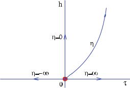
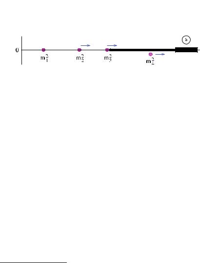
The field theory (2) describes a family of renormalization group trajectories flowing out of the critical point located at h = τ = 0 (Fig. 1). Since the coupling conjugated to an operator Φ has the dimension of a mass to the power 2 − XΦ , the
combination |
τ |
|
|
η = |
(3) |
||
|
|||
|h|8/15 |
is dimensionless and can be used to label the trajectories. In particular, the lowand high-temperature phases at h = 0 and the critical isotherm τ = 0 correspond to η = −∞, +∞, 0, respectively.
Fig. 1 The Ising field theory (2) describes a one-parameter family of renormalization group trajectories (labelled by η) flowing out of the critical point located at τ = h = 0
Particle Decay in Ising Field Theory with Magnetic Field |
175 |
2 Evolution of the Mass Spectrum |
|
Under analytic continuation to imaginary time the euclidean field theory (2) defines a (1 + 1)-dimensional relativistic theory allowing for a particle interpretation.
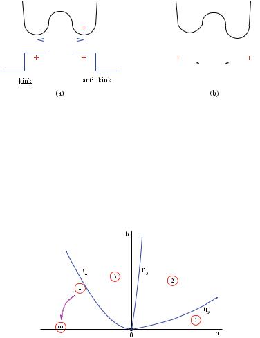
It is well known that the action (2) with h = 0 describes a free neutral fermion with mass m |τ |. While in the disordered phase τ > 0 this fermionic particle corresponds to ordinary spin excitations, in the spontaneously broken phase τ < 0 it describes the kinks interpolating between the two degenerate ground states of the system (Fig. 2a). In the euclidean interpretation the space-time trajectories of the kinks correspond to the domain walls separating regions with opposite magnetization.
A small magnetic field switched on at τ < 0 breaks explicitly the spin reversal symmetry and removes the degeneracy of the two ground states (Fig. 2b). To first
order in h the energy density difference between the two vacua is |
|
E 2h σ , |
(4) |
where σ is the spontaneous magnetization at τ = 0. With the symmetry broken the kinks are no longer stable excitations. An antikink-kink pair, which was a twoparticle asymptotic state of the theory at h = 0, now encloses a region where the system sits on the false vacuum (Fig. 2b). The need to minimize this region induces
an attractive potential |
|
V (R) E R |
(5) |
(R is the distance between the walls) which confines the kinks and leaves in the spectrum of the theory only a string of antikink-kink bound states An, n = 1, 2, . . . , whose masses
mn = 2m + |
(ΔE )2/3zn |
, h → 0 |
(6) |
m1/3 |
are obtained from the Schrödinger equation with the potential (5). The zn in (6) are positive numbers determined by the zeros of the Airy function, Ai(−zn) = 0. This non-relativistic approximation is exact in the limit h → 0 in which mn − 2m → 0. The spectrum (6) was first obtained in [16] from the study of the analytic structure in momentum space of the spin-spin correlation function for small magnetic field. Relativistic corrections to (6) have been obtained more recently1 in [23].
The particles An with mass larger than twice the lightest mass m1 are unstable. It was conjectured in [16] that the number of stable particles decreases as η increases from −∞, until only A1 is left in the spectrum of asymptotic particles as η → +∞. The particle A1 would then be the free fermion of the theory at η = +∞. According to this scenario, for any n > 1 there should exist a value ηn for which mn crosses the decay threshold 2m1, so that the particle An becomes unstable for η > ηn. The natural expectation is that the values ηn decrease as n increases, in such a way that the τ -h plane is divided into sectors with a different number of stable particles as
1 See also [24] which appeared after this talk was given.
176 |
|
|
|
|
|
|
|
|
|
|
|
|
|
|
|
|
|
|
Gesualdo Delfino |
|||
|
|
|
|
|
|
|
|
|
|
|
|
|
|
|
|
|
|
|
|
|
|
|
|
|
|
|
|
|
|
|
|
|
|
|
|
|
|
|
|
|
|
|
|
|
|
|
|
|
|
|
|
|
|
|
|
|
|
|
|
|
|
|
|
|
|
|
|
|
|
|
|
|
|
|
|
|
|
|
|
|
|
|
|
|
|
|
|
|
|
|
|
|
|
|
|
|
|
|
|
|
|
|
|
|
|
|
|
|
|
|
|
|
|
|
|
|
|
|
|
|
|
|
|
|
|
|
|
|
|
|
|
|
|
|
|
|
|
|
|
|
|
|
|
|
|
|
|
|
|
|
|
|
|
|
|
|
|
|
|
|
Fig. 2 The free energy and the kink excitations in the spontaneously broken phase (a). A small magnetic field removes the degeneracy of the ground states and confines the kinks (b)
qualitatively shown in Fig. 3. The trajectories corresponding to the values ηn are expected to densely fill the plane in the limit η → −∞.
This pattern has been confirmed by numerical investigations of the spectrum of the field theory (2) for all values of η [8, 23, 24]. For η → −∞ the particles An with n large can be studied within the semiclassical approximation and their decay widths have been obtained in [19, 24].
Fig. 3 Expected evolution of the mass spectrum as a function of η. In the sector in between ηn and ηn+1 the theory possesses n stable particles (numbers in the circles)
3 Particle Decay off the Critical Isotherm
The critical isotherm η = τ = 0 must lie within the sector in which the theory has, generically, three stable particles (Fig. 3). To understand this we must recall that A. Zamolodchikov showed in [22, 21] that the theory (2) with τ = 0 is integrable and computed its exact S-matrix. He found that the spectrum along this integrable trajectory consists of eight stable particles A1, . . . , A8 with masses
Particle Decay in Ising Field Theory with Magnetic Field |
177 |
|||||||
m1 h8/15 |
π |
|
|
|
|
|
||
m2 = 2m1 cos |
= (1.6180339887..) m1 |
|
||||||
|
|
|
||||||
5 |
|
|
||||||
m3 = 2m1 cos |
π |
|
= (1.9890437907..) m1 |
|
||||
|
|
|
||||||
30 |
|
|||||||
m4 = 2m2 cos |
7π |
|
= (2.4048671724..) m1 |
|
||||
|
|
|
||||||
30 |
|
(7) |
||||||
m5 |
= 2m2 cos |
2π |
|
= (2.9562952015..) m1 |
||||
|
|
|
||||||
15 |
|
|
||||||
m6 |
= 2m2 cos |
π |
|
= (3.2183404585..) m1 |
|
|||
|
|
|
||||||
30 |
|
|
||||||
m7 |
= 4m2 cos |
π |
cos |
7π |
= (3.8911568233..) m1 |
|
||
|
|
|
|
|||||
5 |
|
30 |
|
|||||
m8 |
= 4m2 cos |
π |
cos |
2π |
= (4.7833861168..) m1. |
|
||
|
|
|
|
|||||
5 |
|
15 |
|
|||||
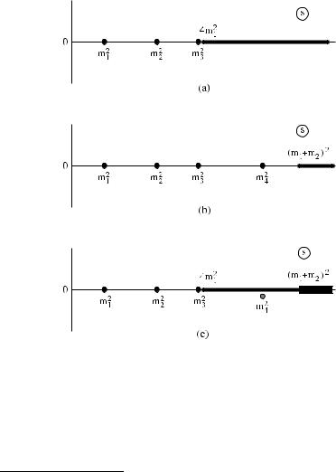
A peculiarity of this spectrum is that only the lightest three particles lie below the lowest decay threshold 2m1. The remaining five have the phase space to decay and certainly are not prevented to do so by internal symmetries (the magnetic field leaves no internal symmetry in the Ising model). It is easy to see that, while there is nothing wrong with the stability of the particles above threshold along this integrable trajectory, they must necessarily decay as soon as a deviation, however small, from the critical temperature breaks integrability [10]. Figure 4 shows the bound state poles and the unitarity cuts of the elastic scattering amplitudes S11 and S12 in the complex plane of the relativistic invariant s (square of the center of mass energy). We know from [22, 21] that at τ = 0 the scattering channel A1A1 produces the first three particles as bound states (Fig. 4a), while the channel A1A2 produces the first four (Fig. 4b). The absence of inelastic scattering in integrable theories allows only for the unitarity cut associated to the elastic processes. When integrability is broken (i.e. as soon as we move away from τ = 0), however, the inelastic channels and the associated unitarity cuts open up. In particular, the process A1A2 → A1A1 acquires a non-zero amplitude, so that the threshold located at s = 4m21 becomes the lowest one also in the A1A2 scattering channel (Fig. 4c). Since the pole associated to A4 is located above this threshold, it can no longer remain on the real axis, which in that region is now occupied by the new cut. The position of the pole must then develop an imaginary part which, according to the general requirements for unstable particles [11], is negative and brings the pole through the cut onto the unphysical region of the Riemann surface. The other particles above threshold, which appear as bound states in other amplitudes at τ = 0, decay through a similar mechanism. We see then that, because of integrability, the trajectory η = 0 corresponds to an isolated case with eight stable particles inside a range of values of η in which only the particles A1, A2, A3 are stable.
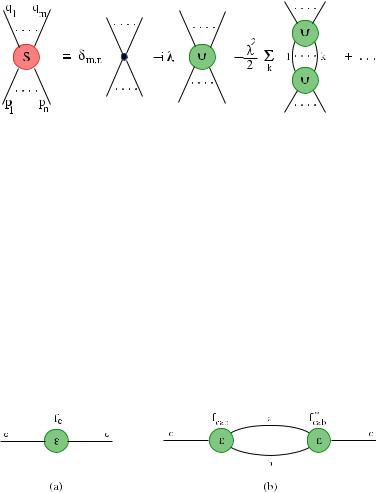
These decay processes associated to integrability breaking can be studied analytically through the form factor perturbation theory around integrable models [8]. Indeed, if the action of the perturbed integrable theory is
178 |
Gesualdo Delfino |
Aintegrable + λ d2x Ψ (x), |
(8) |
the perturbative series in λ can be expressed in terms of the matrix elements of the perturbing operator Ψ on the asymptotic particle states (Fig. 5). These matrix elements can be computed exactly in the unperturbed, integrable theory exploiting analyticity constraints [14, 20] supplemented by operator-dependent asymptotic conditions at high energies [5, 9, 6].
Fig. 4 Poles and unitarity cuts for the elastic scattering amplitudes S11 and S12 in the integrable case τ = 0, (a) and (b), respectively, and for τ slightly different from zero (c). In (c) the particle A4 became unstable and the associated pole moved through the cut into the unphysical region
For our present purposes we then look at the action (2) as the integrable trajectory τ = 0 perturbed by the energy operator ε(x) and must compute corrections in τ . The matrix elements of an operator Φ(x) in the unperturbed theory can all be related to the form factors2
2 The energy and momentum of the particles are parameterized in terms of rapidities as
(p0, p1) = (ma cosh θ , ma sinh θ ).
Particle Decay in Ising Field Theory with Magnetic Field |
179 |
FaΦ1...an (θ1, . . . , θn) = 0|Φ(0)|Aa1 (θ1) . . . Aan (θn) , |
(9) |
where |0 is the vacuum state and the asymptotic states are built in terms of the eight particles which are stable at τ = 0.
Fig. 5 Perturbative expansion for a scattering amplitude in the theory (8). The matrix elements of the perturbing operator Ψ can be computed exactly in the unperturbed, integrable theory
To lowest order in τ the corrections to the real and imaginary parts of the masses come from the perturbative terms in Fig. 6 and are given by [8]
δ Re mc2 −2τ fc, |
|
|
|
(10) |
||
Im mc2 −τ 2 |
21−δab |
|fcab |2 |
|
|
, c = 4, 5 |
(11) |
|
(cab) |
| |
||||
a≤b, ma +mb ≤mc |
|
mc ma | sinh θa |
|
|
||
with |
|
|
|
|
|
|
fc = Fccε (iπ, 0), |
|
|
|
(12) |
||
fcab = Fcabε (iπ, θa(cab), θb(cab)); |
|
|
(13) |
|||
θa(cab) is determined by energy-momentum conservation at the vertices in Fig. 6b.
Fig. 6 Terms determining the leading corrections to the real (a) and imaginary (b) parts of the masses in Ising field theory at small τ . For c > 5 also diagrams with more than two particles in the intermediate state contribute to the imaginary part
The available decay channels for the particles above threshold are determined by the spectrum (7):
180 |
Gesualdo Delfino |
|
A4 → A1A1 |
A5 → A1A1, |
A1A2 |
A6 → A1A1, |
A1A2, A1A3, A1A1A1, |
and similarly for A7 and A8. For c > 5 the sum in (11) must be completed including the contributions of the decay channels with more than two particles in the final state.
Oneand two-particle form factors for Ising field theory at τ = 0 have been computed in [5, 7] (see [4] for a review). Table 1 contains the complete list of oneparticle matrix elements for the relevant operators. The results for the lightest particle are compared in Table 2 with the result of numerical diagonalization of the transfer matrix on the lattice [3]. Three-particle form factors have been computed in [10] in order to determine the imaginary parts (11).
Table 1 One-particle form factors for the operators σ and ε in Ising field theory at τ = 0 [5, 7].
The rescaling implied by the notation ˆ ≡ ensures that the results in the table are universal
Φ Φ/ Φ
|
σˆ |
εˆ |
F1 |
−0.640902.. |
−3.706584.. |
F2 |
0.338674.. |
3.422288.. |
F3 |
−0.186628.. |
−2.384334.. |
F4 |
0.142771.. |
2.268406.. |
F5 |
0.060326.. |
1.213383.. |
F6 |
−0.043389.. |
−0.961764.. |
F7 |
0.016425.. |
0.452303.. |
F8 |
−0.003036.. |
−0.105848.. |
Table 2 Lightest-particle form factors at τ = 0 from integrable quantum field theory [5, 7] and |
||||||||
from numerical diagonalization of the transfer matrix [3] |
|
|
||||||
|
|
|
Field theory |
|
Lattice |
|
||
|
F |
σˆ |
− |
0.640902.. |
− |
0.6408(3) |
|
|
|
|
1 |
|
|
|
|
||
|
F |
εˆ |
− |
3.70658.. |
|
− |
3.707(7) |
|
|
|
1 |
|
|
|
|
||
The available results relevant for the leading mass corrections are |
||||||||
f1 = (−17.8933..) ε |
|f411 |
| = (36.73044..)| ε | |
||||||
f2 = (−24.9467..) ε |
|f511 |
| = (19.16275..)| ε | |
||||||
f3 |
= (−53.6799..) ε |
|f512 |
| = (11.2183..)| ε | |
|||||
f4 |
= (−49.3206..) ε |
|
|
|
|
|||
where ε is taken at τ = 0. The ratios |
|
|
|
|
|
lim |
δ Re ma2 |
|
fa |
|
|
|
= 2 ε , |
(14) |
|||
η→0 δE |
|||||
Particle Decay in Ising Field Theory with Magnetic Field |
181 |
where δE is the variation of the vacuum energy density, are completely universal and particularly easy to check numerically. These predictions for the variations of the real part of the masses of the first four particles have been confirmed numerically both in the continuum [8, 24] and on the lattice [13]. Using the result3 [12]
ε = −(2.00314..)|h|8/15, |
|
(15) |
|||
it easy to check that the sign of the variations |
|
|
|
||
|
τf1 |
fa |
|
|
|
δra = − |
|
ra2 − f1 |
+ O(τ |
2) |
(16) |
m1ma |
|||||
of the mass ratios ra = Re ma /m1 agrees with the McCoy-Wu scenario (Fig. 7).
Fig. 7 Evolution of the mass spectrum as predicted by (16) as τ increases from 0. A2 and A3 approach the threshold and will decay for positive values of τ ; A4 has already become unstable for τ < 0 and moves further away from the threshold
The above values of fabc give [10] |
|
|
|
|
|
|||
Im m42 (−173.747..)τ 2, |
(17) |
|||||||
Im m52 (−49.8217..)τ 2, |
(18) |
|||||||
and in turn the decay widths and lifetimes |
|
|
|
|||||
|
Im m2 |
|
1 |
|
||||
Γa = − |
|
a |
, |
ta = |
|
(19) |
||
|
ma |
Γa |
||||||
of the particles A4 and A5. The lifetime ratio |
|
|
|
|||||
τlim0 |
t4 |
= 0.23326.. |
|
(20) |
||||
t |
|
|
||||||
→ |
|
|
5 |
|
|
|
|
|
is universal, as well as the branching ratio for A5, which decays at 47% into A1A1 and for the remaining fraction into A1A2.
It appears from (20) that A5 lives more than four times longer than A4, somehow in contrast with the expectation inherited from accelerator physics that, in absence of symmetry obstructions, heavier particles decay more rapidly. Notice, however, that in d dimensions the width for the decay Ac → Aa Ab is
3 The value (15) refers to the normalization of ε in which ε(x)ε(0) → |x|−2 as |x| → 0.