Лекции_Микроэкономика

LECTURE NOTES for

INTERMEDIATE MICROECONOMICS

Contents

1. CONSUMER’S THEORY……………………………………………………. 3

1.1Budget constraint…………………………………………………………….. 3

1.2Preferences…………………………………………………………………… 6

1.3Utility………………………………………………………………………… 7

1.4Consumer’s choice…………………………………………………………... 8

1.5Comparative statics and demand…………………………………………….. 10

1.6Alternative approach to consumer’s theory: revealed preferences…………... 12

1.7Price changes: Slutsky decomposition………………………………………. 13

1.8Price changes: Another substitution effect…………………………………... 16

1.9In-kind income……………………………………………………………….. 17

Application: Consumption-leisure model (Individual labour supply)…………… 18

2.INTERTEMPORAL CHOICE……………………………………………….. 27 2.1 Consumption choices over time……………………………………………... 27 2.2 Production and consumption over time: saving and investment…………….. 29 2.3 Applications of NPV rule: non-renewable (or exhaustible) resources………. 31

3.CHOICE UNDER UNCERTAINTY…………………………………………. 35 3.1 Gambles and contingent commodities……………………………………….. 35 3.2 Expected utility………………………………………………………………. 40 Application 1. Obtaining additional information………………………………... 41 Application 2. Insurance…………………………………………………………. 42

Application 3. Diversification…………………………………………………… 43

4.THE FIRM………………………………………………………………….…. 45 4.1 Modeling the firm’s technological opportunities……………………………. 45 4.2 Profit maximization and Cost minimization…………………………………. 46 4.3 Cost minimization……………………………………………………………. 47 4.4 Profit maximization in case of perfect competition…………………………. 53

5.PERFECT COMPETITION AND MONOPOLY…………………………….. 55 5.1 Perfect competition ………………………………………………………….. 55 5.2 Equilibrium and efficiency…………………………………………………... 59 Application: per unit tax analysis………………………………………………... 60

1

5.3Monopoly…………………………………………………………………….. 62

5.4Monopolistic price discrimination…………………………………………… 68 6. STRATEGIC INTERACTIONS……………………………………………… 75

6.1Basic concepts of game theory………………………………………………. 75

6.2 Oligopoly with homogeneous products……………………………………… 76 6.3 Basic concepts of game theory: sequential games…………………………… 79

6.4Dynamic oligopolistic models……………………………………………….. 80

6.5Entry, market structure and strategic entry deterrence………………………. 84

6.6Product Differentiation………………………………………………………. 86 7. FACTOR MARKETS………………………………………………………… 92

7.1Demand for factors…………………………………………………………... 92

7.2The supply of factors and competitive equilibrium………………………….. 96

7.3Monopsony and monopoly in factor markets………………………………... 96

8. GENERAL EQUILIBRIUM AND WELFARE ECONOMICS……………… 99

8.1Pareto efficiency……………………………………………………………... 99

8.2Equilibrium and efficiency…………………………………………………... 103 9. ASYMMETRIC INFORMATION……………………………………………. 106

9.1Hidden characteristics in insurance market………………………………….. 106

9.2Job market signalling (Spence model) ………………………………………. 109

9.3Asymmetric information: hidden actions……………………………………. 110

9.4 Moral hazard in labour markets……………………………………………… 112

10. EXTERNALITIES, PUBLIC GOODS AND PUBLIC CHOICE………… 116

10.1Externalities as a source of market failure………………………………….. 116

10.2Responses to externalities…………………………………………………... 117

10.3Public goods………………………………………………………………... 121

10.4Public choice……………………………………………………………... 122

2

1. CONSUMER’S THEORY

Economists assume that consumers choose the best bundle of goods they can afford.

Thus we have to describe more precisely what we mean by “best” and what we mean by “can afford”. We start with the concept of affordable bundle.

1.1 Budget constraint

Bundlevector of commodities

In an economy with N commodities bundle is described by vector x x1 , x2 , ,xN , where xi stays for the quantity of good i .

Each commodity can be consumed only in nonnegative amount, i.e. xi 0 .

Key assumption. Consumer is a price taker, i.e. price per unit of a commodity is not affected by the number of units purchased.

p1 x1 p2 x2 pN xN or simply px .

Suppose that consumer has money income I , then he can afford all bundles that cost no more than I .

We call the set of all affordable consumption bundles at prices p p1 , p2 , , pN and income I the budget set of the consumer.

Budget set contain bundles x 0 that satisfy the following constraint p1 x1 p2 x2 pN xN I ,

which is called budget constraint.

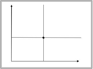
In case of two goods we can illustrate budget set graphically using budget line. Budget line is the set of bundles that cost exactly I : p1 x1 p2 x2 I .

Budget line slope. As x2 ( I p1 x1 ) / p2 , then dx2 p1 . dx1 p2

3

Note:

1)vertical and horizontal intercepts represent bundles in which only one of the commodities is consumed;

2)the slope is equal to negative of the price ratio and reflects the opportunity cost of consuming good 1 (in order to consume more of good 1 you have to give up some consumption of good 2).

Change in the price of good 1 results in rotation of budget line.

I

p2

~

p1 p2

p1

p2

Change in income brings a parallel shift of budget line.

4

p1 p1

2

In-kind transfer of commodity 1, equal to x1

x2

I

x1

5

The numeriare

Budget set is not affected if all prices and income change proportionally. We can divide all prices and income by the price of the second good:

In this case we use second good as a numeriare.

2-goods case

There are more than 2 commodities, but we can treat good 2 as a composite commodity with price equal 1. Then good 2 represents the amount of all other (than good 1) commodities that agent can purchase by spending $1. Notation: AOG

1.2 Preferences

Assumptions

 Completeness: consumer can compare any two bundles and tell, which one he/she prefers or whether he/she is indifferent between them

 Transitivity: for any three bundles x, y, z : if x is preferred to y and y is preferred to z , then x is preferred to z

The set of all bundles that are indifferent to a given bundle is called indifference curve. Implication of transitivity: different indifferent curves do not intersect

Non-satiation: more is better

x2

These bundles are

~

preferred to x

~

x

~x is preferred to these bundles

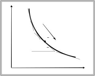
With non-satiation assumption, indifference curves cannot slope upward.

diminishing marginal rate of substitution

6

Marginal rate of substitution of good 1 for good 2 MRS12 (i.e. putting of good 2 in place of

good 1) is the maximum amount of good 2 a person is willing to give up to obtain one additional unit of good 1 or (in the limit) it is the rate at which commodity 2 must decrease as commodity 1 increases by an infinitesimal amount to keep the individual on the same indifference curve.

Diminishing MRS12

x

MRS12 x

Suppose that indifference curve (IC) is described by the function x2 f x1 . Then MRS12 is equal to the absolute value of the slope of IC

Implication of diminishing MRS: convex to the origin ICs

Examples of preferences

Perfect substitutes: goods that can be substituted for each other at a constant rate Perfect complements: goods that have to be consumed in fixed proportions “Bads” (violates the assumption of non-satiation)

1.3 Utility

Utility function is a function that assigns a number to every possible consumption bundle such that more preferred bundles get assigned larger numbers that less preferred bundles.

Denote this function by u .

Note: utility function allows ranking bundles by their amount of utility but it does not allow precise comparisons of how various bundles are valued relative to each other. Such function is called ordinal as it only orders the bundles.

As a result of its ordinal nature utility function is not unique. We can multiply utility by some positive number and get different utility function that represents the same preferences.

In fact we can use any positive monotonic transformation.

7

Examples of utility functions.

Perfect substitutes: u x1 , x2 x1 x2

Perfect complements: u x1 , x2 min x1 , x2

“Bad”: u x1 , x2 x1 x2

Cobb-Douglas utility function: u x1 , x2 x1 x2

How to calculate MRS

Marginal utility of commodity i - change in total utility due to an increase in consumption of

this commodity by additional unit: MU i uxi

This concept allows calculating MRS as a ratio of marginal utilities. IC: u x1 , x2 u .

Question. Check that MRS for g u is the same as MRS for u if g 0 .

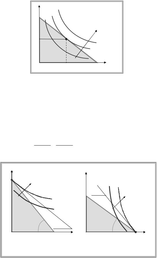
1.4 Consumer’s choice

Utility maximization problem

max u x1 , x2

x1 0, x2 0

p1 x1 p2 x2 m.

Graphical solution

8

x2

Increase in utility

x

Question. Consider any point on budget line where MRS12 p1 / p2 . Explain, why this point is not optimal.

Other interpretation of interior optimum condition: marginal utility per dollar spent has to be

MU1 x MU 2 x . p1 p2

x2

Increase in utility

9

1.5 Comparative statics and demand

Comparative statics - comparison of two equilibria.

Marshallian demand functions x1 p1 , p2 ,I and x1 p1 , p2 ,I -solutions of UMP

Income changes

Normal good - a good for which an increase in income increases consumption ceteris paribus

x2

Income consumption curve

0 x1

Inferior good - a good for which an increase in income decreases consumption ceteris paribus Income elasticity of demandthe percentage change in quantity demanded with respect to a

Own price changes

Derivation of individual’s demand curve

10