Лекции_Микроэкономика

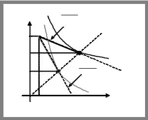
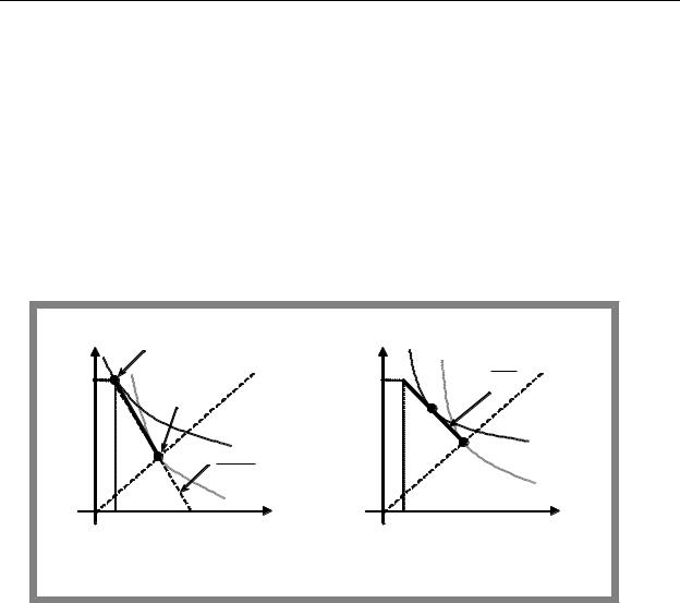
The set of all points efficient in consumption is given by the locus of tangency of agents’ indifference curves and is called contract curve in consumption.

Y A

X B OB

Contract curve

Y

O A X A

X Y B

Efficiency in production

An allocation of inputs is efficient in production if given the total amount of each input available for production, the only way to increase the output of one commodity is to decrease the output of another commodity.

Note that this condition is necessary for Pareto efficiency. Indeed if condition is violated, then by reallocating inputs we can produce more of one good under the same quantity of the other. Let us distribute this additional quantity produced equally between all consumers and each one would be better off, which means that initial allocation was not Pareto efficient.

Let us denote the fixed supply of capital and labour by K and L . Then all feasible allocations could be represented by production Edgeworth box.

L K Y

101

A.Friedman ICEF-2012

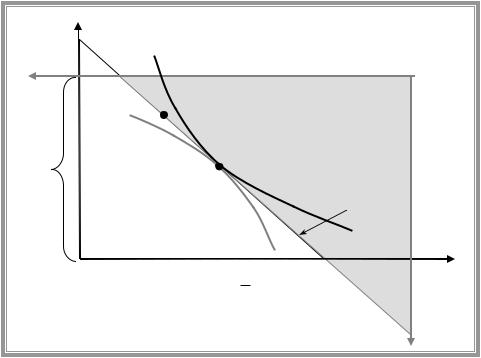
Efficiency in output mix (allocation efficiency)

For allocation efficiency the rate at which producers can convert Y into X has top be equal to the rate at which consumers are willing to sacrifices Y for X: MRTxy MRS xy . Suppose this

is not the case and MRS xy MRTxy , then we should reallocate resources in favor of

good X production as consumers value additional unit of good X more than it costs. Indeed if we produce additional unit of X, the we have to reduce production of good Y by . Let us change the bindle of consumer A leaving bundle of agent B unchanged. Then A will increase his consumption of X by one unit and reduce consumption of Y by but he was willing to

sacrifice up to units of good Y for additional unit of X but actual reduction in consumption of Y was less, which means that he is better off, while welfare of B is unaffected. Thus initial allocation was not PO.

8.2 Equilibrium and efficiency

General equilibrium

A set of prices constitutes general equilibrium if

(1)every firm maximizes profits given its technology,

(2)every consumer maximizes utility subject to his/her budget constraint,

(3)demand equals supply for each commodity.

The First Fundamental Theorem of Welfare Economics

If there is a market for every commodity, optimizing behaviour of consumers and firms under perfect competition leads to a Pareto optimal allocation of resources.

Let us prove that general competitive equilibrium is efficient in consumption, production and output mix.

Equilibrium allocation is feasible as demand for each commodity equals supply.

In equilibrium MRS between the two equals the price ratio. As both consumers face the same prices we get equality of MRS in equilibrium. As each consumer maximizes his utility subject

103

O A X A

X

Y B

As there is no production, this is the only efficiency condition in the economy.

Each firm maximizes profit taking prices as given. Cost minimization is a necessary condition of profit maximization. Cost minimization implies that MRTS between capital and labour in

.

Thus price system allows Pareto efficiency to be achieved in a decentralized setting. No one direct agents to choose particular combinations of inputs or consumption goods. Efficiency arises automatically as the outcome of a process in which each consumer and each producer observes prices and privately makes the decisions that maximize his or her well-being. This is the outcome of

The Second Fundamental Theorem of Welfare Economics

Usually in the economy we have many different PO allocations. Can any arbitrary PO allocation be attained by some set of competitive prices, assuming there is a suitable assignment of initial endowments? The answer to this question is provided by the second welfare theorem.

104

If insurance is fair ( t pt ), then insurance company gets zero profit per dollar of insurance sold and is willing to sell any quantity.

If insurance is favourable ( t pt ), then insurance company gets negative expected profit and is not willing to supply insurance at all.

Finally, if insurance is unfavourable ( t pt ), then each unit of insurance sold brings

positive profit and the solution of profit maximization problem does not exist (supply is unlimited).

Thus the case of unfavourable insurance can never be observed in equilibrium.

Favourable price does not equilibrate market as well since supply is zero, while demand is positive.

It means that equilibrium price has to be fair, i.e. each agent would be insured completely but pieces are different.

Equilibrium under asymmetric information

Suppose that each customer knows his probability of loss, but insurance companies do not know.

As insurance companies are not allowed to differentiate between the two types of customers, there would be one market with uniform price.

insurance (assuming that overinsurance is not allowed), i.e. zH L . Low-risk agents find this price two high and will purchase less than full insurance, i.e. zL L . As the quantity

demanded by good customers (low risk) is less that quantity demanded by high-risk, the resulting expected profit would be negative:

Thus insurance company will never sell insurance under this price. As a result price of insurance goes up and two types of equilibrium may take place.

107

A.Friedman ICEF-2012

Note that, in general, equilibrium price should bring zero expected profit. As negative expected profit results in zero supply, while positive expected profit leads to unlimited supply.

Equilibrium of type 1 corresponds to pH . If low risk agents find this price two high and

prefer to stay at initial endowment, then only high risk stay at the market and purchase full insurance at fair price.

Thus only high risk agents may stay at the market, i.e. we deal with adverse selection problem.

Equilibrium of type 2 corresponds to pav pH . At this price high risk agents purchase

full insurance (as price is favourable) while low risk find the price unfavourable and purchase only partial insurance. Moreover losses of insurance company from high-risk agents are compensated by profit from low-risk so that total expected profit is zero.

Whatever is the equilibrium, risk is allocated inefficiently.

As firms are risk neutral while agents are risk averse at efficient allocation insurance companies should bear all the risk, while agents have to be insured completely. But in equilibrium only high-risk agents are insured completely, while low risk take at least part of the risk.

Responses to adverse selection problem

Private response

group insurance plans (employers offer health insurance as part of benefits. Insurance company deals with group of people and so it faces average risk since agents can’t refuse from purchasing insurance)

targeted insurance rates (insurance premium is based on observable characteristic that is correlated with unobservable one)

signalling (response of informed side)

screening (response of uninformed side)

Government response:

108

compulsory health insurance, compulsory public pension programs, OSAGO (as program is compulsory, insurance company deals with average risk)

information policies:

o prohibiting false advertising, o setting quality standards,

omandatory disclosure of certain facts (used car dealers are supposed to disclose known defects)

9.2Job market signalling (Spence model)

Assumptions:

two groups of workers: high-productive (productivity 400) and low-productive (productivity 200), groups of equal size,

partial employment is not allowed,

price of final product is normalized to 1,

utility is increasing in aggregate commodity ( y ) and decreasing in education ( e ),

the cost of acquiring additional unit of education for low-productive are higher than for high-productive (as a result indifference curves of low-productive workers are steeper)

AOG, y

yL

yHe

e

reservation utility is 0,

output is produced by labour only,

firms treat education as a signal of productivity,

workers choose education first, education is observed by firms

Suppose that firms treat any person with at least bachelor’s degree ( e 4 ) as a high productive one. As a result compensation is 200 if e e and 400 if e e . If under this compensation scheme high-productive maximises utility at e , while low-productive choose different point, then signalling is successful.

109

Conditions of successful signalling:

workers must be able to take some action observable to employers,

cost of such action must be lower for high-productive workers,

cost of action are less than benefit for able workers (he takes the action) but not for unable workers.

Screening

Screening deals with uninformed party’s attempt to sort the informed parties by offering special pricing schemes.

Screening requires some self-selection deviceuninformed party is offered a set of options, and the choice made by the informed party reveals his/her hidden characteristic.

Example. Low insurance premium in case of deductibles and high insurance rates for full insurance (Deductibles: if damage is below certain limit, than agent pays for the bill himself, if damage is above certain limit, then only damage in excess of this limit is compensated).

Low risk agents prefer insurance with deductibles with low insurance premium, while highrisk purchase expensive full insurance.

9.3 Asymmetric information: hidden actions

In situations of hidden action one side of a transaction can take an action that affects the other side but is not observable

Hidden actions may lead to moral hazard problem.

Moral hazard problem - a party to a contract engages in post-contractual opportunistic behaviour, i.e. take the wrong action.

Examples: worker may choose to shirk on a job; an insurance policyholder may fail to take enough care to prevent an accident

Moral hazard in insurance markets

In case of fire insurance an uninsured person can take some actions that reduce the probability of fire (i.e. by properly storing flammables, inspecting gas lines and so on). We will call these activities by word “care”. In the absence of insurance a person will choose the level of care by equating MB of care with MC.

110