

Лекции_Микроэкономика
.pdfA.Friedman |
|
|
|
|
ICEF-2012 |
NOTE: As TC SR VC Q FC , then MC SR |
TC SR |
|
VC Q FC |
|
VC Q . |
|
Q |
|
Q |
|
Q |
Shape of the short-run MC is determined by return to variable factor.
MC SR |
VC Q |
|
wL Q |
w |
L Q |
|
w |
. |
Q |
Q |
Q |
|
|||||
|
|
|
|
MP |
||||
|
|
|
|
|
|
|
L |
|
Conclusion:
MC=const if MPL const ,
MC increases if MPL diminishes in Q,
MC decreases if MPL increases in Q,
Short-run average cost ( AC SR ) - the short-run total cost divided by the number of unites
produced: AC SR TC SR VC Q FC AVC Q AFC , Q Q
where AVC denotes average variable cost: AVC Q VC Q ?
Q
AFC denotes average fixed cost: AFC FCQ .
As FC const , then AFC is diminishing function of output
AFC
0 |
Q |
|
The shape of AVC depends on return to variable factor.
VC Q |
|
wL Q |
|
QL Q wL Q |
|
||||||
|
|
|
|||||||||
AVC Q |
|
|
|
|
|
|
w |
|
|
|
|
|
|
|
|
2 |
|
||||||
|
Q |
|
|
|
Q |
|
|
Q |
|
|
|
|
|
|
|
|
|
|
|
|
|||
w |
L Q |
|
w |
1 |
|||
|
L Q |
|
|
|
|
|
|
|
|
|
|
||||
|
|
Q |
|
|
|
|
MPL |
Q |
|
|
Q |
||||
1
APL
As we can see dynamics of AVC depends on the relationship between average and marginal products of labor.
|
If MPL |
APL , then AVC Q 0 |
, i.e. AVC is constant. |
||
|
If MPL |
APL , then AVC Q 0 |
, i.e. AVC is increasing. |
||
|
If MPL |
APL , then AVC Q 0 , i.e. AVC is diminishing. |
|||
Suppose that |
F |
|
,0 0 , i.e. labour is essential factor. |
||
K |
|||||
The first case takes place if marginal product is constant.
51

A.Friedman |
|
|
ICEF-2012 |
Q |
|
||
F( L ), K |
K |
|
|
|
|
|
MPL APL |
||||
|
|
0 |
|
|
|
|
L |
|
|
|
|
|
|
|
|
The second case takes place if MPL is diminishing. |
|||||||
|
|
Q |
|
|
|
|
|
|
|
K K |
|
|
|||
|
|
|
|
|
|||
|
|
|
|
|
|
|
F( L ) |
|
|
|
|
MPL APL |
|||
|
|
|
|
|
|
|
|
|
|
0 |
APL |
|
|
||
|
|
|
|
|
|
L |
|
|
|
|
|
|
|
|
|
The last case takes place if MPL |
is increasing. |
|
|
||||
|
|
|
|
|
|
||
|
|
Q |
K |
K |
|
F( L ) |
|
|
|
|
|
|
|||
|
|
|
MPL APL |
|
|
||
|
|
|
|
|
|
MPL |
|
|
|
0 |
APL |
|
|
||
|
|
|
|
|
|
L |
|
|
|
|
|
|
|
|
|
|
|
|
|
|
|||
MPL |
AVC |
AFC |
|
AC SR |
|||
constant |
constant |
decreasing |
|
decreasing |
|||
diminishing |
increasing |
decreasing |
|
decreasing at small Q |
|||
|
|
|
|
|
|
|
increasing at large Q |
increasing |
decreasing |
decreasing |
|
decreasing |
|||
NOTE: U-shaped short-run AC appears if MPL is diminishing
Relationships between AVC and short-run MC (the same as for long-run AC and MC)
|
If VC(0)=0, then AVC 0 MC 0 .. |
|
If AVC reaches minimum at Q 0, then AVC Q MC Q , |
|
If AVC diminishes over some range of outputs, then AVC Q MC Q for all Q from |
|
considered range, |
|
52 |
A.Friedman |
ICEF-2012 |
If AVC increases over some range of outputs, then AVC Q MC Q for all Q from considered range.
Exercise. Suppose that AVC, AC and MC are U-shaped and TC(0)=0. Sketch AVC, short-run AC and MC curves on the same graph.
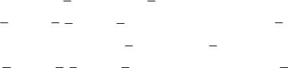
Relationships between the SR and LR cost curves
TC LR Q TC SR Q,K for any Q and K ,
TC LR Q TC SR Q ,K , where K - the level of capital optimal for Q . Implication: AC LR Q AC SR Q,K for any Q and K ,
AC LR Q AC SR Q ,K , where K - the level of capital optimal for Q .
Cost minimization with two plants
Suppose firm has two plants that produce the same output with different technologies. The resulting cost functions are given by TC1 q and TC2 q .
Question: what is the firm’s cost function?
To find out the firm’s cost function we have to allocate any given output Q in a cost minimizing way between the two plants:
TC firm Q min TC1 q1 TC2 q2 . s.t. q1 q2 Q
As q2 Q q1 , then TC firm Q min TC1 q1 TC2 Q q1 .
If both plants are used in production (i.e. we deal with interior solution), then the FOC implies
TC q |
TC |
Q q , i.e. |
MC |
q |
MC |
q |
2 |
. It means that in case when both plants are |
|
1 |
1 |
2 |
1 |
1 |
1 |
2 |
|
|
|
used, output is allocated in such a way that MC of production are equalized. If for some level of Q MC of production at one plant is always less than MC of production of the other plant, then only plant with lowest marginal cost would be used.
4.4 Profit maximization in case of perfect competition
Profit maximization problem max pQ TC w,r,Q .
Q 0
Rules of profit maximization:
1.produce only if Q 0 or p TC / Q TC 0 / Q .
2.if Q 0 , then produce at a point, where p MC Q 0 (First order condition for interior solution);
3.produce at a point, where 0 (Second order condition);
Implications for the long-run:
1. |
produce only if p AC LR Q 0 , i.e. p AC LR Q as TC LR 0 0 . |
2. |
if Q 0 , then produce at a point, where p MC LR Q |
53
A.Friedman |
ICEF-2012 |
3.produce at a point, where MC LR Q  Q 0 , i.e. at non-diminishing part of long-run MC.
Implications for the short run: |
|
1. produce only if p AC SR Q AFC , i.e. |
p AC SR Q AFC AVC Q as |
TC LR 0 FC . |
|
2.if Q 0 , then produce at a point, where p MC SR Q
3.produce at a point, where MC SR Q  Q 0 , i.e. at non-diminishing part of short-run MC.
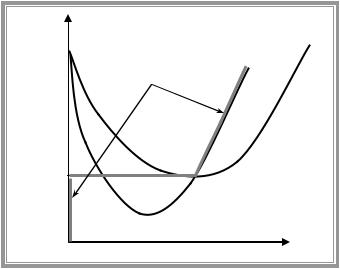
Suppose that AC and MC are U-shaped and TC(0)=0. Let us sketch the long run supply curve.
NOTE: As AC is U-shaped, then p AC LR Q for all p min AC LR Q . As a result we get the following LR supply curve:
|
|
0, |
p min AC LR Q |
|
|
Q |
LR |
|
|
|
|
|
p |
|
|
p min AC LR Q |
|
|
|
Q : |
0, |
||
|
|
MC LR Q p, MC LR Q |
|||
|
|
|
|
|
|
$
AC LR
Firm’s LR supply
min AC |
|
|
MC LR |
0 |
Q |
Consider an example with U-shaped short-run AC, AVC and MC. As AVC is U-shaped, then |
|||
p AVC |
Q |
for all p min AVC Q . As a result we get the following SR supply curve: |
|
Q SR p |
0, |
|
p min AVC Q |
|
|
|
|
|
|
|
|
|
Q : |
MC SR Q p, MC SR Q 0, p min AVC Q |
|
|
|
|
|
54
A.Friedman |
ICEF-2012 |
5. PERFECT COMPETITION AND MONOPOLY
5.1 Perfect competition
Fundamental assumptions of perfect competition
Buyers and sellers are price takers (each agent chooses its actions under the assumption that it cannot influence the prices of the goods)
Entry into the market is free (new suppliers can enter the market without any restrictions on the process of entry)
To find equilibrium market price and quantity we need information about market demand and market supply curves.
Market demand could be obtained by summing up (horizontally) the individual’s demand curves.
p |
p |
|
p |
Q p 20 p, p 10 |
||
|
|
|
|
|||
q1 p 10 p 20 |
q2 p 20 p |
20 |
|
2 p, p 10 |
||
|
|
|
|
30 |
||
|
|
|
|
|
Market demand |
|
10 |
|
|
10 |
|
q1(p)+ q2(p) |
|
|
|
|
|
|
|
|
q1(p) |
|
|
|
|
|
|
|
|
q2(p) |
|
|
|
|
10 |
q1 |
20 q2 |
10 |
|
30 |
Q |
Market supply is different in the SR and in the LR as in the SR new firms cannot enter the market as they cannot obtain the needed fixed inputs. In the LR new firms can enter and existing firms can exit.
The short run
In the SR the number of firms in the industry is fixed and we get SR industry supply by summing up the firms SR supply curves.
As each firm produce at non-diminishing part of its MC the resulting SR industry supply is upward sloping. The result does not depend on whether suppliers are homogeneous (have the same cost functions) or heterogeneous (have different cost functions).
p |
p |
|
p |
|
q s p |
q s |
p |
pb |
1 |
2 |
|
|
|
|
SR Industry supply
p a
|
a |
b |
q1 |
a |
|
b |
q2 |
q |
a |
q |
a |
q |
b |
q |
b |
Q |
q |
q1 |
q2 |
q |
|
2 |
|
2 |
|||||||||
|
|
2 |
|
1 |
|
1 |
|
|
||||||||
1 |
|
|
|
|
|
|
|
|
|
|
|
|
|
|
||
55

A.Friedman |
ICEF-2012 |
Market is in equilibrium if:
(1)buyers are choosing their optimal purchase levels, given the prevailing market price;
(2)sellers are choosing their optimal output levels, given the prevailing market price;
(3)suppliers are willing to produce as much as buyers wish to purchase.
SR equilibrium corresponds to the intersection of market demand with SR industry supply. Equilibrium price p is a solution of the equation QD p QS p .
p
Industry supply
p
|
Market demand |
Q |
Q |
The long run
In the LR new suppliers can enter the market and old suppliers can exit.
To know the market quantity supplied at a given price, we need to find both the quantities supplied by each firm in the market and the number of suppliers who choose to be in the market at that price.
(a) homogenous firms
We start with homogenous firms case, i.e. the case, where all firms have identical cost functions.
Consider the constant cost industry- industry, where individual firm’s cost function remains unchanged as industry output expands.
Note, that as all firms have the same technology, nobody is willing to produce at price that is below the minimum of AC. Thus quantity supplies is zero at any price below p min AC . Now, let us take any price above min AC . At this price pa AC qa
profit. New firms will be attracted to the industry by the prospect of earning positive economic profit (due to assumption of constant cost industry the expansion of industry output have no effect on cost curves of individual firm). Thus industry supply is unlimited at this
price. The same argument applies for any other price that exceeds p . If p min AC , then each firm produces q and gets zero economic profit. Thus firm is indifferent between being
in and out of the market. Thus with any number of firms in the industry there is no incentive to enter or exit the market. Thus any quantity can be produced.
56

A.Friedman |
|
|
ICEF-2012 |
p |
|
p |
|
MC LR |
|
Constant cost industry |
|
AC LR |
|
|
|
p a |
|
|
|
p |
|
|
LR Supply |
|
|
|
|
|
|
|
Q D |
q q a |
q |
Q |
Q |
Firm |
|
Market |
|
Conclusion: in case of constant-cost industry LR industry supply is zero for p min AC and is horizontal at p min AC .
As a result the quantity produced by the industry is determined by the market demand and the number of firms in the industry N we get as a ratio of industry and individual output:
p min AC , Q QD p , q arg min AC q , N Q / q .
Note: firm’s output corresponding to the minimum of AC is called minimum efficient scale.
Looking at the LR equilibrium we assumed that an increase in the industry output has no effect on individual firm cost function. It may not be the case. We can observe both external diseconomies (an increase in industry output brings an increase in LRAC) or external economies (an increase in industry output results in a reduction in LRAC). There are two reasons for the presence of external economies/diseconomies:
(1)pecuniary external economy/diseconomy is a result of interaction between industry output and firm’s cost function through the changes in the market prices of inputs;
(2)technological external economy/diseconomy is a result of interaction between industry output and firm’s cost function through the physical possibilities of production (i.e. the production function).
Examples: pecuniary diseconomy may result from increased competition for specific factor; technological economy may come from innovations that represent a by-product of an increased industry output.
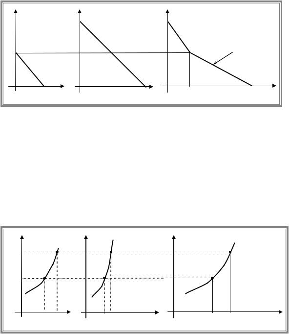
Increasing cost industry - an industry in which external diseconomies take place, i.e. LRAC rise with the industry output level.
The LR industry supply will be upward sloping as min AC LR rises with expansion in industry output. Note: although min AC LR rise with increase in Q , the minimum efficient scale may stay constant, fall or rise.
Decreasing cost industry- an industry in which external economies take place, i.e. LRAC fall as industry output rises.
The LR industry supply will be downward sloping as min AC LR falls with expansion in industry output. Note: although min AC LR falls with increase in Q , the minimum efficient scale may stay constant, fall or rise.
57
A.Friedman |
ICEF-2012 |
p |
p |
|
LR Supply |
p |
p |
|
|
|
|
|
LR Supply |
|
Q D |
|
Q D |
Q |
Q |
Q |
Q |
Increasing cost industry |
Decreasing cost industry |
||
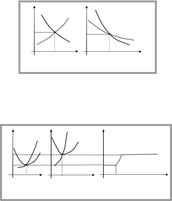
(b) heterogeneous firms
Let us assume that industry output has no effect on the firms cost functions, i.e. we deal with constant cost industry.
Suppose that there are two types of producers of some good. Producers of type 1 have lower costs but the number of type 1 producers is limited (for example they use specific resource with restricted access). Assume for simplicity that there is only one firm of type 1. Producers of type 2 have higher costs of production but any firm can become a type 2 producer.
p |
p |
|
LR |
|
p |
|
|
|
MC2 |
|
|
|
|
MC LR |
|
|
|
|
|
|
|
1 |
|
|
|
|
|
|
AC LR |
|
|
AC2LR |
|
LR Industry supply |
|
|
|
|
|
|
|
p |
1 |
|
|
|
|
|
|
|
|
|
|
|
|
2 |
|
|
|
|
|
|
p |
|
|
|
|
|
|
1 |
|
|
|
|
|
|
q |
q1 |
q |
|
q2 |
|
Q |
|
||||||
1 |
|
2 |
|
|
|
|
Type 1 firm |
|
|
Type 2 firm |
|
|
Market |
In If price is below the minimum of LRAC of the first firm (firm with the lowest cost of production), then nobody is willing to produce at all. As a result industry supply is zero for any p p1 min AC1LR . If price is below the min AC2LR but above min AC1LR other firms are
would be willing to produce had they access to the technology used by firm 1, but the access is restricted firm1 will be the only producer and the industry supply corresponds to the part of MC of firm 1 (if there are more firms of type 1, we should sum up their supply curves for any
p p1 , p2 ). As price reach the level of min AC2LR , then any type 2 firm is able to produce but its profit would be 0. Thus it is indifferent between coming in and staying out. As a result industry supply is horizontal at p2 min AC2LR .
Conclusion: industry supply can be upward sloping even in case of constant cost industry if firms have different cost functions.
58
A.Friedman |
ICEF-2012 |
5.2 Equilibrium and efficiency
We want to know not only how a competitive market works but also whether the results are “good” for the society.
We will use the concept of total surplus (TS) to measure the market performance.
TS is a difference b/w social benefit (measured by total willingness to pay) and social cost.
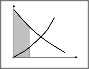
Total willingness to pay (or gross consumers’ surplus) gives total benefit from consumption of given quantity of a good. Graphically it can be represented as an area below the market
demand function. For example if Q Q0 , then total benefit is represented by grey area:
CS gross Q0 A B .
Total cost can be represented as an area below the market supply curve for given number of firms in the industry (integral from MC). If Q Q0 , the cost of production are given by dashed area (B). As a result TS=(A+B)-B=A.
p
Supply
A
Demand
B
Q
Q 0
Another approach to TS.
Note that in the absence of government intervention TS can also be calculated as a sum of net consumers’ surplus (CS) and producers’ surplus (PS). PS is the revenue the agent receives in excess of what he would require to produce a given quantity. If additional unit of output is produced that costs increase by the value of MC, thus the difference b/w market price and MC corresponds to net gain of producer from this additional unit. By summing up over all units produced, we get the PS. Note that in the absence of fixed cost PS is equal to profit.
If we implement this approach, then consumers will purchase Q0 units of output at price p0 (note that at this price producers are willing to supply more than Q0 so that p0 does not
correspond to equilibrium). The resulting CS is an area below the demand function above the market price (grey) and together with PS we get exactly the same value of TS as before.
59
A.Friedman |
ICEF-2012 |
p
Supply
CS
p 0
PS
Demand
Q
Q 0
The key question is whether TS is maximized at competitive equilibrium. If some other allocation had a higher TS, then output would be called inefficient because it would be possible to make society better off.
Claim: competitive equilibrium is efficient.
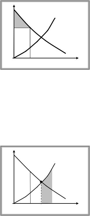
To prove this claim let us look at output level, Qa , which is less than competitive. Then by moving from Qa to Q , total benefit increase by (C+D), while costs increase only by D and TS goes up by C, which implies that initial allocation was inefficient.
Similarly if we look at output level that exceeds equilibrium one, Qb Q , then we can increase TS by moving from Qb to Q as total benefit falls by F, while costs goes up by (E+F). As a result TS is increased by E.
p
Supply
C E
D F |
Demand |
Q
Qa Q Qb
Implication: as competitive equilibrium output is efficient, then any government interventions that result in deviation from competitive output would reduce total surplus, i.e. the corresponding output would be inefficient. The corresponding reduction in TS is called deadweight losses.
Application: per unit tax analysis
Suppose that per unit tax with tax rate of supply curves be linear. Let us denote by
t on sales of good X is introduced. Let demand and p the price paid by consumers and suppose that tax
is paid by producers, then the price received by producers is p t . As a result the FOC in
profit maximization problem looks like p t MC q or |
p MC q t . Thus this tax can |
|
60 |