

Лекции_Микроэкономика
.pdfA.Friedman |
|
|
|
|
|
ICEF-2012 |
|
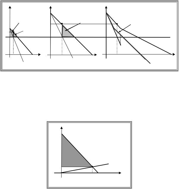
As in both cases output is the same, TS segm TS monopoly |
since under market segmentation |
||||||
output is inefficiently allocated among consumers. |
|
|
|||||
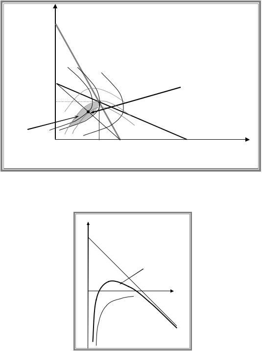
Graphical proof for the case with 2 groups |
|
|
|
||||
p |
|
|
p |
|
p |
|
|
|
|
|
p2(q) |
|
|
|
|
|
|
|
psegm |
DWLsegm2 |
|
MR1+MR2 |
|
|
|
|
|
|
|
||
|
|
|
2 |
|
|
|
|
p mon |
DWL1mon |
|
p mon |
|
p mon |
Market |
|
|
segm |
|
|
|
demand |
|
|
segm |
|
|
|
|
|
||
DWL1 |
|
|
|
|
|
|
|
p1 |
|
MR2 |
|
MR |
|
|
|
|
|
|
|
|
|||
|
|
|
DWLmon2 |
|
|
|
|
|
p1(q) |
|
|
MC=c |
|
||
|
|
|
|
|
|
||
|
q1mon q1segm |
q1 |
q2segm |
q2mon |
q2 |
Qmon Qsegm |
Q |
|
MR1 |
|
|
|
|
|
|
Claim 2. If one group of consumers is not served under uniform price but is served under discrimination, then TS segm
As Qmon |
qmon , then MRtotal Qmon MR |
qmon c . |
|
|
|
|
||||||||
|
2 |
|
|
|
|
|
2 |
2 |
|
|
|
|
|
|
At the |
same |
time |
MR q segm c , |
which implies |
that |
qmon q segm |
but |
|||||||
|
|
|
|
|
2 |
2 |
|
|
|
|
2 |
2 |
|
|
Qmon qmon qsegm qsegm qsegm |
Qsegm |
as by assumption q segm |
0 . |
|
|
|
||||||||
|
2 |
2 |
2 |
1 |
|
|
1 |
|
|
|
|
|||
Market |
|
|
|
|
Pure monopoly |
|
Comments |
|
|
|
|
|||
segmentation |
|
|
|
|
|
|
|
|
|
|
|
|
|
|
q1segm |
|
|
|
> |
|
q1mon |
|
|
|
q1segm >0 and q1mon =0 |
|
|
|
|
q2segm |
|
|
|
= |
|
q2mon |
|
|
|
|
|
|
|
|
Q segm |
|
|
|
> |
|
Qmon |
|
|
|
|
|
|
|
|
Psegm |
|
|
|
< |
|
Pmon |
|
|
Due to diminishing demand |
|
|
|||
CS1segm |
|
|
|
> |
|
CS1mon |
|
|
As q1segm >0 and q1mon =0 |
|
|
|||
CS2segm |
|
|
|
= |
|
CS2mon |
|
|
As q2segm q2mon > |
|
|
|
||
profit |
|
|
|
> |
|
profit |
|
|
Monopolist |
|
under |
|
|
|
|
|
|
|
|
|
|
|
|
|
segmentation |
could |
charge |
|
|
|
|
|
|
|
|
|
|
|
|
the same price as pure |
|
|
||
|
|
|
|
|
|
|
|
|
|
monopolist |
but |
chooses |
|
|
|
|
|
|
|
|
|
|
|
|
different pricing policy |
|
|
||
TS=CS1+CS2+profit |
|
> |
|
TS=CS1+CS2+profit |
|
|
|
|
|
|||||
71
A.Friedman |
|
|
|
|
|
|
ICEF-2012 |
||
p |
|
|
p |
|
|
|
|
p |
|
|
|
|
|
p2(q) |
|
|
|
|
|
|
|
DWL1mon |
psegm pmon |
|
|
DWLsegm2 |
DWLmon2 |
|
|
|
|
2 |
|
|
|
MR1+MR2 |
|||
p1segm |
|
DWL1segm |
|
|
|
|
|
|
|
|
|
|
p mon |
|
|
|
|
|
MC=c |
|
|
|
|
|
|
|
MR |
|
|
|
|
|
|
|
|
|
|
Market |
|
|
|
|
p1(q) |
|
|
MR2 |
|
|
demand |
|
|
|
|
|
|
|
|
|
|
q segm |
q1 |
q |
segm q mon |
q2 |
Qmon |
Q |
|||
|
1 |
MR1 |
2 |
2 |
|
|
|
||
|
|
|
|
|
|
|
|
|
|
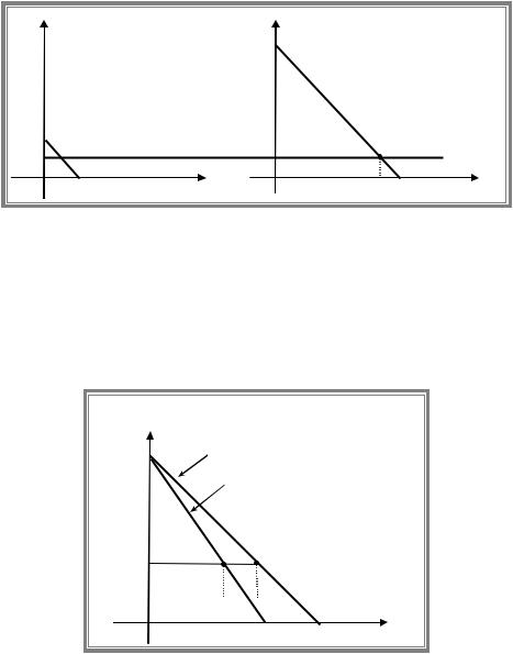
Multi-part pricing: two-part tariff
In a two-part tariff each consumer pays a fixed fee ( F ) for consuming any units at all plus a price per unit ( p ) for each unit consumed.
If there is only one consumer, then for each per unit price p the maximum fee equals to his CS. Thus firm is able to appropriate TS. As a result firm finds optimal to set linear price p MC q and F CS q . As a result firm’s output is efficient.
|
p(q) |
|
F |
p |
MC |
q
q
If there are two consumers with identical demand functions, then solution is very similar. We should find aggregate demand and set p MC Q
which is the same for each consumer.
But if consumers have different demand functions, then we need to establish different fees and in addition monopolist has to be able to identify the type of consumer.
Even in case of heterogeneous customers and unique two-part tariff monopolist may find optimal to set linear part of the tariff equal to MC.
This is the case if monopolist faces with two (equal) groups of customers with large difference in the marginal willingness to pay. Then it is more profitable to deal with high valuation group only (see figure below).
72
A.Friedman |
ICEF-2012 |
p
p2(q)
F
p1(q)
MC
q1 |
q2 |
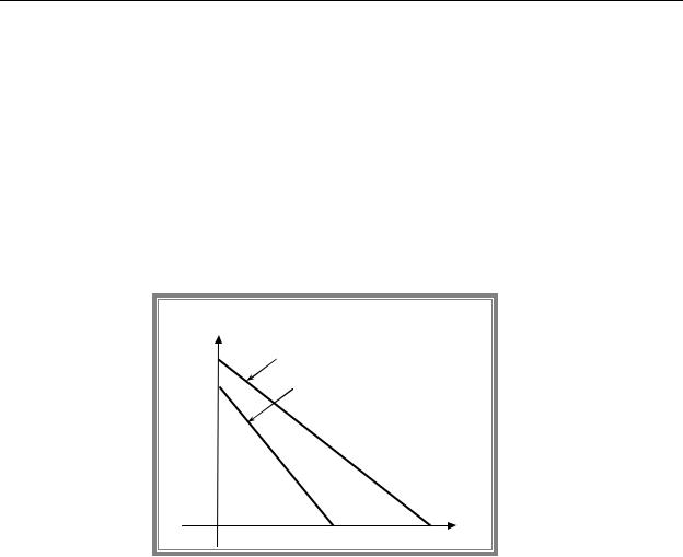
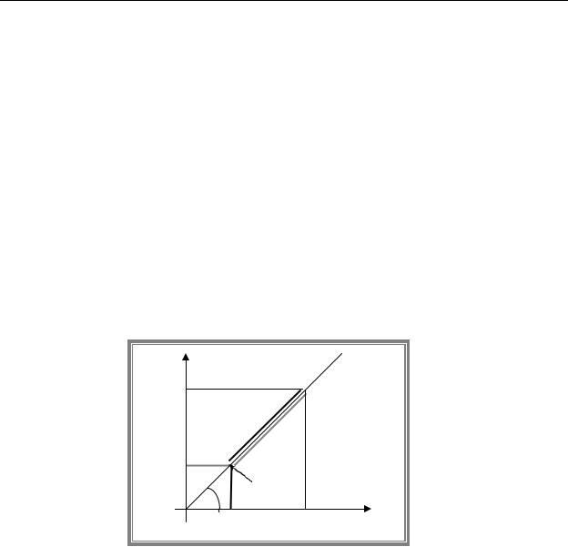
Another possibility corresponds to the situation, when the difference in marginal willingness to pay is not so large as in previous example, but the number of customers with higher marginal willingness to pay is much bigger than the number of buyers with lower willingness to pay.
Now, let us assume that we deal with two groups of equal size and the difference in willingness to pay is not two high. Let us illustrate that monopolist will benefit from charging linear price above marginal cost.
p |
p2(q) |
|
|
|
|
|
|
|
|
|
|
p1(q) |
|
|
|
A |
C |
|
|
~ |
|
|
|
|
p |
|
|
|
|
p0 |
B |
D E |
F |
MC |
|
|
|
q |
|
|
|
|
|
|
First of all we can show that it is more profitable to deal with both groups of consumers rather than only with high valuation one. The optimal tariff in case of selling to highest valuation (i.e. second) group only is to set linear price equal to MC (as a result profit from sales is zero) and fee, equal to the corresponding value of consumer surplus: p0 MC and
F0 A B C D F E . Resulting profit equals to the value of fee: 0 F0 .
If the monopolist will decrease fee up to the value of CS of group 1 ( F A B D ) under the same linear price, his profit will increase: 2F 2( A B D ) 0 as A B D C E F . So he will sell to both groups.
Now, we can illustrate that it is not optimal to set price equal to MC. If monopolist increases |
|||||||||||
linear |
price |
to |
~ |
and |
sets |
~ |
A, |
then |
his |
profit |
equals |
p |
F |
||||||||||
~ 2A B B D E ( E D ) . So, it is profitable to raise linear price above MC.
Second-degree price discrimination
In reality no firm can observe every individual buyer’s willingness to pay for its product. In this case a monopolist can use the consumer’s own actions as a basis of discrimination.
73
A.Friedman ICEF-2012
Second-degree price discrimination - is the practice in which the same price schedule is offered to all buyers but they sort themselves through self-selection.
Example with bundling. Suppose we have two groups with linear demands but the second group has higher willingness to pay (see graph below). For simplicity let’s assume that we have one agent in each group and MC=0. Each consumer knows his/her willingness to pay but monopolist cannot identify the type of each customer.
Had the types been observable as we know from the previous discussion monopolist would sell under linear price equal to MC (zero in this case) and charge fees equal to values of individual’s CS: Fee1 A and Fee2 A B С . In this case monopolist’s profit would be
2A B С . In fact he can achieve the same profit by bundling: if he offers to the first group
bundle with q units at price of |
A |
and to the second group bundle q |
units at price of |
1 |
|
2 |
|
A B С the outcome would be the same.
p
P2(q)
P1(q)
A |
B |
|
|
|
|
|
|
C |
|
|
q |
|
q |
q2 |
|
1 |
|
But as the type are unobservable monopolist is unable to implement this scheme. Now he has to offer the same bundles to every customer. There is no sense to offer the two bundles found above as high valuation agent would definitely take the bundle designed for group one as it gives him net CS of B and monopolist’s profit would go down to 2A . In fact monopolist can still earn more by changing the contract designed for consumer 2 in such a way that consumer would find optimal to choose it. Then this contract should provide agent 2 net CS not less
than B . This can be done by reducing the contract for the large package with q2 units to A C . In this case each consumer self-selects by choosing the contract designed for his/her type and monopolist’s profit would be 2A C . Is it the maximum possible profit? No, we can change the package designed for group 1 to make it less attractive for the second group.
You |
are |
asked |
to |
check |
that the |
optimal |
bundles |
would |
be |
q |
that |
solves |
the |
equation |
||||
P q 2P q |
|
|
|
|
|
q |
|
1 |
|
|
|
|
||||||
with |
price |
equal |
to |
CS |
and |
q |
with |
price |
||||||||||
2 |
|
1 |
1 |
1 |
q |
CS q . |
|
|
1 |
1 |
|
|
2 |
|
|
|||
CS |
2 |
q |
CS |
2 |
|
|
|
|
|
|
|
|
|
|
||||
|
1 |
|
|
1 |
1 |
1 |
|
|
|
|
|
|
|
|
|
|
||
74
A.Friedman |
ICEF-2012 |
6. STRATEGIC INTERACTIONS
6.1 Basic concepts of game theory
If there are several firms in the industry and firms recognize their mutual interdependence, then each firm while choosing price or output takes into account how its rivals will react, that is it behaves strategically.
A situation of strategic interactions is called a game. To specify a game we have to identify
players (the decision makers);
strategies (choices available for each player);
payoffs (the rewards enjoyed by each player at the end of a game).
Example. Prisoners’ Dilemma.
Two prisoners who were partners in a crime were being questioned in separate rooms. Each can either confess to the crime (and thereby implicate the other) or deny his participation in the crime.
If only one prisoner confessed, then he would go for free and the other would spend 6 months in prison. If both denied, then each would spend one month in prison (time required for investigation) and if both confessed, then each would spend 3 months in a prison.
Note that each player would be better off by choosing strategy “confess” whatever is the strategy chosen by the other as 0>-1 and -3>-6. If one strategy gives higher payoffs no matter what any other player does, this strategy is called dominant. Thus in Prisoners Dilemma each player would choose strategy confess. In this case we say that the game has dominant strategies equilibrium. Note, that the outcome of this equilibrium is inefficient as both agents would be better off by playing (Deny, Deny). But (Deny, Deny) outcome can not be achieved as players are unable to cooperate.
Player A |
Deny |
Confess
Player B
Deny Confess
-1,-1 |
-6, 0 |
0, -6 -3, -3
Often we face with a game where there are no dominant strategies. In this case the optimal choice of one player depends on the strategy chosen by the other. We will say that a pair of strategies constitutes a Nash equilibrium if A’s choice is optimal given B’s choice and B’s choice is optimal given A’s choice (i.e. each players choice is a best response for the rivals’ strategy).
Player A |
Top |
Bottom
|
Player B |
|
Left |
|
Right |
2, 1 |
|
0, 0 |
0, 0 |
|
1, 1 |
In this game “Left” is best response for “Top” as 1>0 and “Top” is best response for “Left” as
2>0. Thus (Top, Left) is Nash equilibrium.
75
A.Friedman |
ICEF-2012 |
Similarly “Right” is best response for “Bottom” as 1>0 and “Bottom” is best response for “Right” as 1>0. Thus (Bottom, Right) is another Nash equilibrium.
Note: this section was extended in the new UOL subject guide. You are expected to know both pure and mixed strategies NE.
6.2 Oligopoly with homogeneous products
We start our analysis of oligopolistic markets by looking at firms that compete with homogeneous products.
The Cournot model.
Assumptions:
firms compete by setting quantities,
firms make their choice simultaneously,
firms produce homogeneous product,
entry into the market is completely blocked.
We are going to look at the simplest example of Cournot model with two firms (i.e. the case of duopoly) and assume that both firms have identical CRS technologies (cost function TC q cq ) and market demand is linear p Q A Q , where A c .
To find Nash equilibrium we need to derive the best response function for each firm. But as the two firms have identical technologies, the corresponding best response functions would be symmetric.
The best response function of firm 1 we get as a solution of its profit maximisation problem, where rival’s output is treated as exogenous parameter:
max A q1 q2 q1 cq1 .
q1
As q2 is exogenous, then firm 1 maximizes its profit with respect to residual demand given by q1 p Q p q2 A p q2 , which gives the residual inverse demand function
pres q1 A q1 q2 . The first order condition requires equality of the marginal revenue of firm 1 and its marginal cost:
MR1 q1 A 2q1 q2 c ,
which implies the following best response function of firm 1 |
q |
q |
|
|
A c |
|
q2 |
. Similarly, |
|||||||
2 |
|
|
|||||||||||||
|
|
|
|
|
1 |
|
|
2 |
2 |
|
|||||
|
|
|
|
|
|
|
|
|
|
|
|||||
the best response function of firm 2 is given by |
q |
|
q |
A c |
|
q1 |
. As Nash equilibrium |
||||||||
2 |
|
|
|||||||||||||
|
|
1 |
2 |
|
|
2 |
|
|
|
|
|
|
|||
|
|
|
|
|
|
|
|
|
|
|
|
||||
requires both firms to play the best response strategy, equilibrium quantities are obtained as a solution of the following system
|
|
|
A c |
|
|
|
q1 |
|
|
q2 |
|
||
|
|
|||||
|
|
|
2 |
|
2 . |
|
|
|
|
|
|||
|
|
|
A c |
|
q1 |
|
q2 |
|
|
|
|||
2 |
2 |
|
||||
|
|
|
|
|
||
76
A.Friedman |
|
|
ICEF-2012 |
Thus, in equilibrium q q A c / 3 , Q q q 2 A c / 3 , |
|||
1 |
2 |
1 |
2 |
p A Q A 2c / 3 and A c 2 |
/ 3. |
|
|
|
i |
|
|
We can illustrate equilibrium graphically as an intersection of the two best response functions.
q2
A c q1 q2
|
|
A c |
|
|
|
|
|
Cartel |
|
|
||
|
2 |
|
|
NE |
|
|
|
|
||||
|
|
|
|
|
|
|
|
|
||||
q |
A c |
|
|
|
|
|
|
|
|
|
||
|
|
|
|
|
|
|
|
|
|
|
||
2 |
3 |
|
|
|
|
|
|
|
|
|
||
|
|
|
|
|
|
q2 q1 |
|
|
|
|||
|
|
|
|
|
|
|
|
|
|
|
||
Both firms get |
|
A c |
|
A c |
A c |
|
|
|
||||
higher profit |
q1 |
|
|
|
q1 |
|||||||
3 |
|
|
|
|
|
|||||||
2 |
|
|
|
|
||||||||
|
|
|
|
|
|
|
|
|
||||
Isoprofit lines of firm 1. Equation A q1 q2 q1 cq1 |
1 or q2 |
A c q1 |
|
1 |
||||||||
q1 |
||||||||||||
|
|
|
|
|
|
|
|
|
|
|||
|
|
|
|
|
|
|
|
|
straightline |
|
|
|
hyperbola
q2
A-c
A-c-q1
A c q1 / q1
q1
/ q1
Note, that profit of firm 1 increase as we move down along its reaction curve (i.e. when competitor’s output falls and as a result market price goes up).
Point of maximum of iso-profit curve always lie on the reaction function. The reason is simple: for any output of the competitor (firm 2) the profit maximising output of firm 1 is given by the corresponding point on reaction function and any other output results in lower profit and so should lie on the higher iso-profit line.
77
A.Friedman |
ICEF-2012 |
As we can see both firms can get higher profits by producing less (shaded area). Thus we have a problem similar to prisoners’ dilemma: if firms could collude, they would benefit from the collusion.
Collusion.
If the total output is chosen collectively by the two firms (rather than individually), i.e. firms create a cartel and choose the output by maximising joint profit, then
max A Q Q cQ .
Q
The first order condition requires equality of market marginal revenue with marginal cost, which implies MR Q A 2Q c and Qcartel A c / 2 A c / 3 QCournot.
Note that as both firms have identical CRS technologies the total output can be produced at any plant. Suppose the cartel’s profit is split equally and q1Cartel q2Cartel A c / 4 . This
point is illustrated on the above diagram. Note that cartel solution is characterized by a tangency of the firms’ isoprofit lines.
Comparison of Cournot Duopoly, competition and monopoly.
Cournot Duopoly: QCournot 2 A c / 3, |
pCournot A Q |
A 2c / 3 . |
||||||
Monopoly (collusion): QM A c / 2 , |
pM A c / 2 . |
|
||||||
Perfect competition: Qcomp A c , pcomp c . |
|
|||||||
QM |
|
A c |
QCournot |
2 A c |
A c Qcomp |
|
||
|
|
|
||||||
|
2 |
|
3 |
|
|
|
||
and |
pM pCournot pcomp . |
|
|
|||||
As a result TS M |
TS Cournot TS comp . |
|
|
|||||
Question. Consider Cournot model with N identical firms with |
AC MC c . Suppose that demand |
|||||||
function is linear |
P Q A Q . Find the Cournot-Nash equilibrium and show that monopoly is a |
|||||||
special case of with N 1 and perfectly competitive outcome corresponds to the case of N .
Price-setting oligopolists: Bertrand model
Assumptions:
firms compete by setting prices,
firms make their choice simultaneously,
firms produce homogeneous product,
entry into the market is completely blocked,
each firm has CRS technology, i.e. MC=AC=c.
We start with a classical duopoly model with symmetric firms, that is the case, where MC1 MC2 c . As a result the best response functions would be symmetric.
78
A.Friedman ICEF-2012
|
0 if |
|
pi p j |
|
|
|
|
|
|
Residual demand of firm i = |
Q p |
i |
/ 2 if |
|
p |
i |
p |
j |
. |
|
|
|
|
|
|
|
|||
|
|
|
if pi |
p j |
|
|
|||
|
Q pi |
|
|
||||||
Let us consider the best response of firm i |
to any price chosen by firm j : |
||||||||
If firm j charges price less or equal MC , than the best response is to charge price,
equal to MC (or higher). If firm i responds by lowering the price it will keep all the market and incur losses as price is below its marginal costs.
If firm j charges price above MC but less (or equal) to P Monopoly, then it is optimal to undercut this price by and serve all the market. In this case profit from each unit sold is positive as price is above MCi .
If firm j charges price that exceeds the monopolist one, then firm i responds by
setting the monopolist price. This policy allows to attract all the customers and get the maximum possible (monopolist) profit.
These best response functions are illustrated below.
|
|
p2 |
|
|
|
|
|
|
|
|
|
|
|
pmonopoly |
|
|
|
|
|
|
|
|
|
|
|
|
|
|
|
|
|
|
|
|
|
|
||
|
|
|
|
|
|
|
|
|
|
|
||
|
|
p1 |
( p2 ) |
p2 |
( p1 ) |
|
|
|
|
|||
|
|
|
|
|
|
|
|
|||||
|
MC |
|
|
|
|
|
|
|
|
|
|
|
|
|
|
Nash equilibrium |
|
|
|
|
|||||
|
|
45 |
|
|
|
|
|
|
p1 |
|
|
|
|
|
MC |
|
|
p |
monopoly |
|
|
|
|||
|
|
|
|
|
|
|
|
|||||
|
|
|
|
|
|
|
|
|
|
|
||
~ |
~ |
MC , . As a result firm |
|
|
|
~ |
~ |
~ |
/ 2 |
|||
Nash equilibrium: p1 |
p2 |
1 serves all the market q1 |
q2 |
Q p |
||||||||
and profit of each firm equals zero.
Conclusion: price competition is more severe than quantity competition. The reason is that with identical products a firm that charges lower price takes all the market (not just part of the market).
6.3 Basic concepts of game theory: sequential games
Up until now we have been looking at games in which all players move simultaneously. But in many situations one player gets to move first and the other players responds.
If there are several firms in the industry and firms recognize their mutual interdependence, then each firm while choosing price or output takes into account how its rivals will react, that is it behaves strategically.
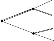
Example. Game tree (game in extensive form)
79
A.Friedman |
|
|
ICEF-2012 |
|
|
left |
(1, 0) |
|
B |
|
|
|
|
|
|
Top |
|
right |
(3, 1) |
A |
|
|
|
Bottom |
B |
left |
(2, 6) |
|
|||
|
|
||
|
|
right |
(9, 0) |
In this game if A plays “Top”, then the best response of B is to play “right” as 1>0. If A plays “Bottom”, then the best response of B is “left” as 6>0. Now let us think about A’s choice. Taking into account the best responses of player B he finds optimal to play “Top” as 3>2. The resulting equilibrium is (Top; (right if top, left if bottom)). Note that we specify the possible actions of the player in every decision node (including those that are not reached in a game). The concept of equilibrium used in this example corresponds to perfect Nash equilibrium that is given by set of strategies that constitute Nash equilibrium in every subgame (i.e. starting from any decision node).
Note that for player the resulting gain equals 1, while he could get 6 had he convinced the other player that he will respond by playing “left” in case of “Top”. But the threat to play “left” is noncreadible as it is not in the interest of B to play “left” as it gives 0 while “right” allows to get 1. Thus the key property of Nash equilibrium is that each player takes into accounts only credible threats.
To find perfect Nash equilibrium (in the finite game) we can use backward induction.
6.4 Dynamic oligopolistic models
The Stackelberg model.
Assumptions:
firms compete by setting quantities,
firms make their choice sequentially,
firms produce homogeneous product,
entry into the market is completely blocked.
In the Stackelberg model one firm, the leader, sets its output first and the other firm (or firms) reacts. This is an example of sequential game an we will look for the perfect Nash equilibrium that requires to use backward induction.
The leader use it first mover advantage by forcing the rival to produce the quantity that combined with the leaders output results in a most profitable outcome for the leader.
To find equilibrium we need to derive the best response function of the follower. Let firm 1
be the leader and firm 2 –the follower. If we use the same assumptions about demand function |
||||||||||||
and |
technologies |
as |
in |
Cournot |
model ( P Q A Q, |
ACi MCi |
c A ), then the |
|||||
reaction function |
of |
the |
follower |
is exactly the same |
is the one |
in Cournot model: |
||||||
q |
|
q |
A c |
|
q1 |
. |
|
|
|
|
|
|
2 |
|
|
|
|
|
|
|
|||||
|
|
1 |
2 |
2 |
|
|
|
|
|
|
||
|
|
|
|
|
|
|
|
|
|
|||
|
|
|
|
|
|
|
|
|
|
|
|
80 |