Patterson, Bailey - Solid State Physics Introduction to theory

Table 7.7. The character table of D3

Below we summarize some important rules for constructing the character table for the irreducible representations. These results will not be proved, since they are readily available.29 These rules are:

1.The number of classes s in the group is equal to the number of irreducible representations of the group.

2.If ni is the dimension of the ith irreducible representation, then ni = χi(E), where E is the identity of the group and ∑sl ni2 = h, where h is the order of the group G. For small finite groups, this rule obviously greatly restricts what the ni can be.

3.If Bk is the number of group elements in the class Ck, then the characters for each class obey the relationship

∑s = Bk χ(l) (Ck )χ( j) (Ck ) = hδ j , k 1 l

where δlj is the Kronecker delta. This relation is often called the orthogonality relation for characters.

4.Suppose the order of a group element g is m (i.e. suppose gm = E). Further suppose that the dimension of a representation (which need not be irreducible) is n. It then follows that χ(g) equals the sum of n, mth roots of unity.

5.The one-dimensional representation is always present.

Finally it is worth giving the criterion for determining the irreducible representations in a given reducible representation. The rule is if

then C′i (which is the number of times that irreducible representation i appears in the reducible representation R) is given by

where χ denotes character relative to R and the sum over k is a sum over classes. When a reducible representation is expressible in the form (7.288) it is said to be in, reduced form. Putting it into such a form as (7.288) is called reduction.

29 See Mathews and Walker [7.47].

448 7 Magnetism, Magnons, and Magnetic Resonance

A frequent use of these results occurs when the representation R is formed by taking direct products (see Sect. 1.2.1 for a definition) of the representations R(i). We can then evaluate (7.289) by remembering that the trace of a direct product is the product of the traces.

There are many ways that group theory has been used as an aid in actual calculations. No doubt there remain other ways that have not yet been discovered. The basic ideas that we will use in our physical calculations involve:

1.The physical system determines a symmetry group with irreducible representations that can be found by group theory.

2.Except for what is called by definition “accidental degeneracy” we have a distinct eigenvalue for each (occurrence of an) irreducible representation. (It is possible for the same irreducible representation to occur many times. The meaning of the word “occur” will be given later.)

3.The dimension of the irreducible representation is the degeneracy of each corresponding eigenvalue.

For a brief insight into the above, let the eigenfunctions of H corresponding to the eigenvalue En be labeled ψni(i → 1 to d). En is thus d-fold degenerate. Thus

It can be shown that Cni matrices are a representation of the group G. We thus have the desired connection between energy levels, degeneracy, and representations.

Let us consider the physically interesting problem of an atom with one 4f electron. Let us place this atom in a potential with trigonal symmetry. The group appropriate to trigonal symmetry is our old friend D3. We want to neglect spin and discover what happens (or may happen) to the 4f energy levels when the atom is placed in a trigonal field. This is a problem that could be directly attacked by perturbation theory, but it is interesting to see what type of statements can be made by the group theory.

If you think a little about the ideas we have introduced and about our problem, you should come to the conclusion that what we have to find is the irreducible representations of D3 generated by (in previous notation) ψ(4f)i. Here i runs from 1 to 7. This problem can be solved by using (7.289).

The first thing we need to know is the character of our rotation group. This is given by [61] for the lth irreducible representation

In (7.294), φ is an appropriate rotation angle. Since we are dealing with a 4f level we are interested only in the case l = 3:

Table 7.13. Character table for calculating Ci′

We can now construct Fehler! Verweisquelle konnte nicht gefunden werden.. Applying (7.289) we have

C1′ = 16 [(7)(1)(1) + 2(+1)(1) + 3(−1)(1)] =1,

C2′ = 16 [7(1)(1) + 2(+1)(1) + 3(−1)(−1)] = 2,

C3′ = 16 [7(1)(2) + 2(+1)(−1) + 3(−1)(0)] = 2 .

Thus

By (7.297) we expect the 4f level to split into two doubly degenerate levels plus three nondegenerate levels. The two levels corresponding to R(3) that occur twice and the two R(2) levels will probably not have the same energy.

450 7 Magnetism, Magnons, and Magnetic Resonance

7.5 Brief Mention of Other Topics

7.5.1 Spintronics or Magnetoelectronics (EE)30

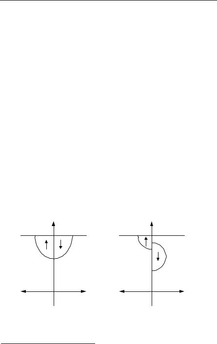
We are concerned here with spin-polarized transport for which the name spintronics is sometimes used. We need to think back to the ideas of band ferromagnetism as contained for example in the Stoner model. Here one assumes that an exchange interaction can cause the spin-up and spin-down density of states to split apart as shown in the schematic diagram (for simplicity we consider that the majority spinup band is completely filled). Thus, the number of electrons at the Fermi level with spin up (Nup) can differ considerably from the number with spin down

(Ndown). See (7.242) and Fig. 7.32 (spins and moments have opposite directions due to the negative charge of the electron – the spins are drawn in the bands). This

results in two phenomena: (a) a net magnetic moment, and (b) a net spin polarization in transport defined by

Fe, Ni, and Co typically have P of order 50%.

In the figures, the D(E) describe the density of states of up and down spins. As shown also in Fig. 7.33 one can use this idea to produce a “spin valve,” which preferentially transmits electrons with one spin direction. Spin valves have many possible device applications (see, e.g., Prinz [7.55]). In Fig. 7.33 we show transport from a magnetized metal to a magnetized metal through a nonmagnetic metal.

Fig. 7.32. Exchange coupling causes band ferromagnetism. The D are the density of states of the spin-up and spin-down bands. EF is the Fermi energy. Adapted from Prinz [7.55]

30 A comprehensive review has recently appeared, Zutic et al [7.73].

452 7 Magnetism, Magnons, and Magnetic Resonance

when the layers are magnetized in the same direction, the spin-dependent scattering is small, and when the layers are alternatively magnetized in opposite directions, the electrons experience a maximum of spin-dependent scattering (and hence much higher resistivity). Thus, magnetoresistance can be used to read the state of a magnetic bit in a magnetic disk drive. The direction of soft layer in the read head can be switched by the direction of the magnetization in the storing media. The magnetoresistance is thus changed and the direction of storage is then read by the size of the current in the read head. Sandwiches of Co and Cu can be used with the widths of the layers typically of the order of nanometers (a few atoms say) as this is the order of the wavelength of electrons in solids. More generally, magnetic multilayers of ferromagnetic materials (e.g. 3d transition metal ferromagnets) with nonferromagnetic spacers are used. The magnetic coupling between layers can be ferromagnetic or antiferromagnetic depending on spacing. Stuart Parkin of IBM has been a pioneer in the development of the GMR hard disk drive [7.52]

Magnetic Tunnel Junctions (MTJs) (EE)

Here the spacer in a sandwich with two ferromagnetic layers is a thin insulating layer. One difficulty is that it is difficult to make thin uniform insulators. Another difficulty, important for logic devices, is that the ferromagnetic layers need to be ferromagnetic semiconductors (rather than metals with far more mobile electrons than in semiconductors) so that a large fraction of the spin-aligned electrons can get into the rest of the device (made of semiconductors). GaMnAs and TiCoO2 are being considered for use as ferromagnetic semiconductors for these devices.

The tunneling current depends on the relative magnetization directions of the ferromagnetic layers. It should be mentioned here that in the usual GMR structures the current typically flows parallel to the layers (but electrons undergo a random walk, and sample more than one layer so GMR can still operate), while in a MTJ sandwich the current typically flows perpendicular to the layers.

For the typical case, the resistance of the MTJ is lower when the moments of the ferromagnetic layers are aligned parallel and higher when the moments are antiparallel. This produces tunneling magnetic resistance TMR that may be 40% or so larger than GMR. MTJ holds out the possibility of making nonvolatile memories.

Spin-dependent tunneling through the FM-I-FM (ferromagnetic-insulator-ferro- magnetic) sandwich had been predicted by Julliere [7.34] and Slonczewski [7.61].

Colossal Magnetoresistance (EE)

Magnetoresistance (MR) can be defined as

where ρ is the resistivity and H is the magnetic field.

454 7 Magnetism, Magnons, and Magnetic Resonance

“Kondo Effect,” pp. 162-165 in [24] and references contained therein. Using quantum dots as artificial atoms and studying them with scanning tunneling microscopes has revived interest in the Kondo effect. See Kouwenhoven and Glazman [7.41].

7.5.3 Spin Glass (A)

Another class of order that may occur in magnetic materials at low temperatures is spin glass. The name is meant to suggest frozen in (long-range) disorder. Experimentally the onset of a spin glass is signaled by a cusp in the magnetic susceptibility at Tf (the freezing temperature) in zero magnetic field. Below Tf there is no long-range order. The classic examples of spin glasses are dilute alloys of iron in gold (Au:Fe, also Cu:Mn, Ag:Mn, Au:Mn and several other examples). The critical ingredients of a spin glass seem to be (a) a competition among interactions as to the preferred direction of a spin (frustration), and (b) a randomness in the interaction between sites (disorder). There are still many questions surrounding spin glasses such as do they have a unique ground state and if the spin glass transition is a true phase transition to a new state (see Bitko [7.7]).

For spin glasses, it is common to define an order parameter by summing over the average spin’s squared:

and for T > Tf, q = 0, while q ≠ 0 for T < Tf. Much further detail can be found in Fischer and Hertz [7.22]. See also the article by Young [7.8 pp. 331-346].

Randomness and frustration (where two paths linking the same pair of spins do not have the same net effective sign of exchange coupling) are shared by many other systems besides spin glasses. Or another way of saying this is that the study of spin glasses fall in the broad category of the study of disordered systems, including random field systems (like diluted antiferromagnets), glasses, neural networks, optimization and decision problems. Other related problems include combinatorial optimization problems, such as the traveling salesman problem, and other problems involving complexity. For the neural network problem see for example, Muller and Reinhardt [7.50]. The book by Fischer and Hertz, already mentioned has a chapter on the physics of complexity with references. Another reference to get started in this general area is Chowdhury [7.12]. Mean-field theories of spin glasses have been promising, but there is no general consensus as to how to model spin glasses.

It is worth looking at a few experimental results to show real spin glass properties. Figure 7.34 shows the cusp in the susceptibility for CuMn. The true Tf occurs as the ac frequency goes to zero. Figure 7.35 shows the temperature dependence of the magnetization and order parameter for CuMn and AuFe. Figure 7.36 shows the magnetic specific heat for two CuMn samples.

456 7 Magnetism, Magnons, and Magnetic Resonance

Fig. 7.36. Magnetic specific heat for CuMn spinglasses. The arrows show the freezing temperature (susceptibility peak). Reprinted with permission from Wenger LE and Keesom PH, Phys Rev B 13, 4053 (1976). Copyright 1976 by the American Physical Society

7.5.4 Solitons31 (A, EE)

Solitary waves are large-amplitude, localized, stable propagating disturbances. If in addition they preserve their identity upon interaction they are called solitons. They are particle-like solutions of nonlinear partial differential equations. They were first written about by John Scott Russell, in 1834, who observed a peculiar stable shallow water wave in a canal. They have been the subject of much interest since the 1960s, partly because of the availability of numerical solutions to relevant partial differential equations. Optical solitons in optical fibers are used to transmit bits of data.

Solitons occur in hydrodynamics (water waves), electrodynamics (plasmas), communication (light pulses in optical fibers), and other areas. In magnetism the steady motion of a domain wall under the influence of a magnetic field is an example of a soliton.32

In one dimension, the Korteweg–de Vries equation

∂u + A ∂3u + B ∂ (u2 ) = 0 ∂t ∂x3 ∂x

(with A and B being positive constants) is used to discuss water waves. In other areas, including magnetism and domain walls, the sine-Gordon equation is encountered

31See Fetter and Walecka [7.20] and Steiner, “Linear and non linear modes in 1d magnets,” in [7.14, p199ff].

32See the article by Krumhansl in [7.8, pp. 3-21] who notes that static solutions are also solitons.