

Higher_Mathematics_Part_2
.pdf2.1.25. а) z = 3x4 y5 + 5x − 2 y4 + 2 ; |
b) z = |
|
ln(x − y) |
. |
|
||||
|
|
|
|||||||
|
|
|
|
|
|
ln(x3 + y3 ) |
|
||
2.1.26. а) z = 4x−2 y−3 − 5x − 4y5 + 8 ; |
b) z = |
ln ln(x ctg y) |
. |
||||||
|
|||||||||
|
|
|
|
|
|
x2 |
|
||
2.1.27. а) z = 9x−2 y6 + 3x4 − 2y + 3 ; |
b) z = |
|
sin 2 x − cos2 y . |
||||||
2.1.28. а) z = − x2 y−3 + 8y3 + 6x −1 ; |
b) z = |
|
tg2 x + ctg2 |
y . |
|||||
2.1.29. а) z = 3x3 y5 − 6xy2 + 2x − 7 ; |
b) z = sin(ln(2x + 3y)) . |
||||||||
2.1.30. а) z = 4x3 y7 + 4xy2 + 4y − 6 ; |
b) z = ln cos(4x − 3y) . |
||||||||
2.2. Find the differential dz for the given functions z(x, y) |
at point М. |
||||||||
2.2.1. |
x + 2 y + z + ez = 0 , M (1; − 1; 0) . |
|
|
|
|
|
|
|
|
2.2.2. |
x2 − y + z + ln z = 0 , M (0; 1; 1) . |
|
|
|
|
|
|
|
|
2.2.3. sin(x + y) + sin( y − z) = 1 , M (0; π / 2; π / 2) . |
|
||||||||
2.2.4. sin(x + y + z) + z = 1 , M (π / 4; π / 4; 0) . |
|
||||||||
2.2.5. e x+ z + e y+ z = 2 , M (0; 0; 0) . |
|
|
|
|
|
|
|
||
2.2.6. 2xy + yz + z3 = 0 , M (−1; 1; 1) . |
|
|
|
|
|
|
|
||
2.2.7. |
xyz + e z = x , M (1; 2; 0) . |
|
|
|
|
|
|
|
|
2.2.8. |
x − y − z = tg z , M (2; 2; 0) . |
|
|
|
|
|
|
|
|
2.2.9. e xyz = z , M (0; 1; 1) . |
|
|
|
|
|
|
|
||
2.2.10. |
ln z + ln x = y − 1, M (1; 1;1) . |
|
|
|
|
|
|
|
|
2.2.11. xyz = ln z , M (0; 1; 1) . |
|
|
|
|
|
|
|
||
2.2.12. |
x + 4y − z = e z , M (−3; 1; 0) . |
|
|
|
|
|
|
|
|
2.2.13. sin z + cos(x − y + z) = 1 , M (π / 2; π / 2; 0) . |
|
||||||||
2.2.14. 3 x + 3 y + 3 z = 4z , M (8; 1; 1) . |
|
|
|
|
|
|
|||
2.2.15. tg x + tg y + tg z = 2 cos z , M (π / 4; π / 4; 0) . |
|
||||||||
2.2.16. |
x2 − y 2 − z 2 + xz + 4x + 5 = 0 , M (−2; 1; 0) . |
|
|||||||
2.2.17. |
x2 + y 2 − z 2 + xz + 4 y − 4 = 0 , |
M (1; 1; 2) . |
|
||||||
2.2.18. 2x2 − y 2 + 2z 2 + xy + xz − 3 = 0 , |
M (1; 2;1) . |
|
|||||||
2.2.19. 4y2 − z2 + 4xy − xz + 4z − 10 = 0 , |
M (1; − 2;1) . |
|
|||||||
2.2.20. |
x2 − 2y 2 + z 2 + xz − 4y − 13 = 0 , |
M (3; 1; 2) . |
|
||||||
|
|
31 |
|
|
|
|
|
|
|
http://vk.com/studentu_tk, http://studentu.tk/
2.2.21. |
y2 + z2 + x − 3z = 0 , M (1; 1;1) . |
|||
2.2.22. |
y 2 + z 2 − xy − z( y + x) = 0 , |
M (1; 2;1) . |
||
2.2.23. 2(x4 + y 4 + z 4 ) − 3xyz = 0 , |
M (1/ 2;1/ 2; 1/ 2) . |
|||
2.2.24. sin 2 x + sin 2 y + sin 2 z − 1 = 0 , M (π / 4; 0; π / 4) . |
||||
2.2.25. ex + e y |
+ ez |
= 3ex+ y+ z , M (0; 0; 0) . |
||
2.2.26. esin x + esin y |
+ ecos z − 3 = 0 , |
M (0; 0; π / 2) . |
||
2.2.27. |
xy + yz |
+ zx |
− 12 = 0 , M (3; |
2; 1) . |
2.2.28. |
x3 + y3 + z3 + xyz − 4 = 0 , M (1; 1; 1) . |
|||
2.2.29. |
x + |
y + |
z + xyz − 8 = 0 , |
M (1;1; 4) . |
2.2.30. 2x + 2 y + 2z + 1 = 2x+ y+ z , |
M (0; 1; 2) . |
|
|
|
|||
2.3. Use the differential to estimate the given expressions. |
|||||||
2.3.1. (0,97)4 (0,95)−2 . |
2.3.2. (0, 94)2 (0, 98)−3 . |
||||||
2.3.3. |
(3,1)2 + (3,9)2 . |
2.3.4. 3 (1,94)3 + (4,06)2 + 3 . |
|||||
2.3.5. sin 5° cos80° . |
2.3.6. sin 6° tg 48° . |
||||||
2.3.7. |
sin 8° + 4 cos 5° . |
2.3.8. |
(5, 85)2 + (8,1)2 . |
||||
2.3.9. |
(4, 75)2 + (11, 8)2 . |
2.3.10. |
arctg |
1, 08 |
. |
||
|
|||||||
|
|
|
|
|
1, 04 |
|
|
2.3.11. tg 42° tg 50° . |
2.3.12. sin 27° cos 4° . |
||||||
2.3.13. |
(2,94)3 − (1,2)2 − 1 . |
2.3.14. |
4 (6, 9)2 + (4, 8)2 + 7 . |
||||
2.3.15. |
sin 85° + 3cos 6° . |
2.3.16. e0,15 (3,05)−2 . |
|||||
2.3.17. sin 6° cos 8° . |
2.3.18. e0,1 sin 85° . |
||||||
2.3.19. |
arctg |
1,1 |
. |
2.3.20. arctg(0, 97 1, 08) . |
|||
|
|||||||
|
0, 96 |
|
|
|
|
|
|
2.3.21. |
4 (2,9)2 + (2,05)2 + 3 . |
2.3.22. 5 (2,9)4 − (3,86)3 + 15 . |
|||||
2.3.23. ((1,86)3 + (0,94)3 )2 . |
2.3.24. 3 (2,05)4 − (3,04)2 + 1 . |
||||||
2.3.25. (1,04)3 (0,96)−1/ 3 . |
2.3.26. ctg 40° ctg 47° . |
||||||
2.3.27. ctg 41° + ctg 51° . |
2.3.28. 5 (4,92)2 + (2,94)2 − 2 . |
||||||
|
|
|
|
32 |
|
|
|
http://vk.com/studentu_tk, http://studentu.tk/

Topic 3. Applications of partial derivatives
Tangent plane and normal to a surface. Directional derivatives and the gradient. Relative extrema of the functions of two variables. Extrema on a polygon.
Literature: [3, ch. 6, §3], [4, section 6, § 20], [6, ch. 6], [7, section 8, §§14––18], [9, §§45––46].
|
|
Т.3 |
|
Main concepts |
|
|
||
|
|
|
|
|
|
|||
|
3.1. Tangent plane and normal to a surface |
|
|
|||||
|
Consider a surface that is a level surface of a function u = F(x, y, z). Let |
|||||||
M0(x0, y0, z0) be a point on this surface where the vector F = |
∂F(M 0 ) |
i + |
||||||
|
||||||||
|
∂F(M0 ) |
|
|
∂F(M0 ) |
|
∂x |
||
+ |
|
j + |
k ≠ 0. The tangent plane to the surface at the point M0 |
|||||
|
|
∂y |
|
∂z |
|
|
||
is that plane through M0 that is perpendicular to the vector F evaluated at M0.
The tangent plane at the point M0 is the plane that best approximates the surface near M0. It consists of all the tangent lines at M0 to curves in the surface that pass through the point M0.
A straight line is perpendicular to a surface at the point M0 on this surface if the straight line is perpendicular to the tangent plane at the point M0, is called the normal line and the following table lists 1.1 and 1.2 have the equations of a tangent plane and a normal line.
|
|
|
|
|
|
|
|
|
|
|
|
|
|
|
|
|
|
|
|
|
|
|
|
|
|
|
|
|
|
|
|
|
Table list 1.1 |
|
|
|
|
|
|
|
|
|
|
|
|
|
|
|
|
|
|
|
|
|
|
|
|
|
|
|
|
|
|
|
|
|
|
|
|
The equations |
|
|
|
|
|
|
|
|
The equations of a tangent plane |
|
|
|||||||||||||||||||||||
of a surface |
|
|
|
|
|
|
|
|
|
|
||||||||||||||||||||||||
|
|
|
|
|
|
|
|
|
|
|
|
|
|
|
|
|
|
|
|
|
|
|
|
|
|
|
|
|
|
|
|
|
|
|
F(x, y, z) = 0 |
|
∂F(M0 ) |
(x − x0 ) + |
∂F(M0 ) |
( y − y0 ) + |
|
∂F(M0 ) |
(z − z0 ) = 0 |
|
|||||||||||||||||||||||||
|
∂x |
|
|
|
|
|
|
|
|
|
|
∂z |
|
|||||||||||||||||||||
|
|
|
|
|
|
|
|
|
|
∂y |
|
|
|
|
|
|
|
|
|
|
|
|
|
|
|
|||||||||
z = f (x, y) |
|
z − z |
0 |
= |
|
|
∂f (x0 , y0 ) |
|
(x − x ) |
+ |
∂f (x0 , y0 ) |
|
( y − y ) |
|
||||||||||||||||||||
|
|
|
|
|
|
|
|
|
|
|||||||||||||||||||||||||
|
|
|
|
|
|
|
∂x |
|
|
|
|
|
0 |
|
|
|
|
|
|
|
|
∂y |
0 |
|
||||||||||
|
|
|
|
|
|
|
|
|
|
|
|
|
|
|
|
|
|
|
|
|
|
|
|
|
|
|
|
|||||||
|
|
|
|
|
|
|
|
|
|
|
|
|
|
|
|
|
|
|
|
|
|
|
|
|
|
|
|
|
|
|
|
|
Table list 1.2 |
|
|
|
|
|
|
|
|
|
|
|
|
|
|
|
|
|
|
|
|
|
|
|
|
|
|
|
|
|
|
|
|
|
|
|
|
The equations |
|
|
|
|
|
|
|
|
The equations of a normal line |
|
|
|||||||||||||||||||||||
of a surface |
|
|
|
|
|
|
|
|
|
|
||||||||||||||||||||||||
|
|
|
|
|
|
|
|
|
|
|
|
|
|
|
|
|
|
|
|
|
|
|
|
|
|
|
|
|
|
|
|
|
|
|
F(x, y, z) = 0 |
|
|
|
|
|
|
|
|
x − x0 |
|
= |
|
y − y0 |
|
|
|
= |
|
|
|
|
z − z0 |
|
|
||||||||||
|
|
|
|
|
|
|
|
|
|
|
|
|
|
|
|
|
|
|
|
|
|
|
|
|
|
|
|
|
||||||
|
|
|
|
|
|
|
∂F(M0 ) |
|
|
|
|
|
∂F(M0 ) ∂F(M0 ) |
|
|
|||||||||||||||||||
|
|
|
|
|
|
|
|
|
|
|
|
|
|
|
||||||||||||||||||||
|
|
|
|
|
|
|
|
|
∂x |
|
|
|
|
|
|
|
|
∂y |
|
|
|
|
|
|
|
|
|
∂z |
|
|
|
|||
|
|
|
|
|
|
|
|
|
|
|
|
|
|
|
|
|
|
|
|
|
|
|
|
|
|
|
|
|||||||
z = f (x, y) |
|
|
|
|
|
|
|
|
x − x0 |
|
|
|
= |
|
|
y − y0 |
|
|
|
|
= |
z − z0 |
|
|
||||||||||
|
|
|
|
|
|
∂f (x0 , y0 ) |
∂f (x0 , y0 ) |
|
−1 |
|
|
|
||||||||||||||||||||||
|
|
|
|
|
|
|
|
|
∂x |
|
|
|
|
|
|
|
|
∂y |
|
|
|
|
|
|
|
|
|
|
|
|
||||
|
|
|
|
|
|
|
|
|
|
|
|
|
|
|
|
|
|
|
|
|
|
|
|
|
|
|
|
|
|
|
|
|||
|
|
|
|
|
33 |
|
|
|
|
|
|
|
|
|
|
|
|
|
|
|
|
|
|
|
|
|
|
|||||||
http://vk.com/studentu_tk, http://studentu.tk/
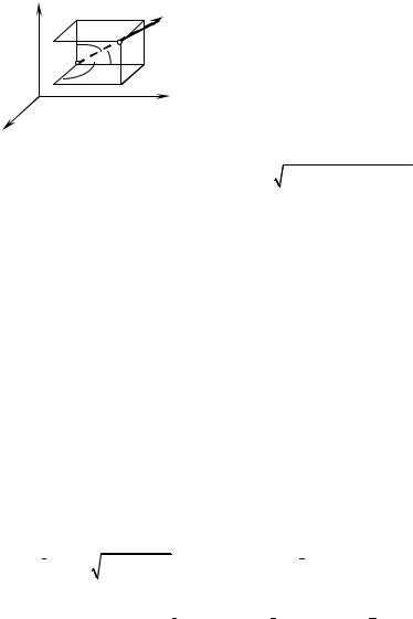
3.2. The directional derivatives and gradient of f(x, y, z)
|
|
z |
|
|
|
|
|
|
|
|
Let a function u = f (x, y, z) be defined and |
|||||||||||||||||
|
|
|
|
М1 |
|
|
continuous a nearby point M(x0, y0, z0). There is |
|||||||||||||||||||||
|
|
|
|
|
М γ |
|
|
l |
|
a unit vector l |
= {cosα; cosβ; cosγ} at М (α, β |
|||||||||||||||||
|
|
|
|
|
|
β |
|
|
and γ are angles with x-, y- and z-axes respec- |
|||||||||||||||||||
|
|
|
|
|
α |
|
|
|
|
|
|
|
tively). A point M1(x0 + |
x, y0 + y, z0 + z) lies |
||||||||||||||
|
|
|
О |
|
|
|
|
|
y |
|
on the straight line which passes though M in the |
|||||||||||||||||
|
|
|
|
|
|
|
|
|
direction |
of |
the vector |
|
|
l (fig. 1.12). |
The |
|||||||||||||
|
x |
|
|
|
Fig. 1.12 |
|
|
distance |
|
l |
between M and M1 by the |
|||||||||||||||||
|
|
|
|
|
|
|
Pythagorean theorem, |
|
|
|
|
|
|
|
|
|||||||||||||
|
|
|
|
|
|
|
|
|
|
|
|
|
|
|
|
l = ( x)2 + ( y)2 + ( z)2 . |
|
|
|
|||||||||
|
|
|
|
|
|
|
|
|
|
|
||||||||||||||||||
|
|
|
Directional derivative of a function u(x, y, z). The derivative of u at |
|
|
|||||||||||||||||||||||
|
|
|
M(x0, y0, z0) in the direction of the unit vector l (it is denoted |
∂u |
|
) is |
|
|
||||||||||||||||||||
|
|
|
∂l |
|
|
|||||||||||||||||||||||
|
|
|
|
|
|
|
|
|
|
|
|
|
|
|
|
|
|
|
|
|
|
|
|
|
|
|
||
|
|
|
|
|
|
|
|
|
∂u |
= lim |
|
u = |
lim |
u(M1 )−u(M ) |
|
|
|
|
||||||||||
|
|
|
|
|
|
|
|
|
∂l |
|
|
|
|
|
||||||||||||||
|
|
|
|
|
|
|
|
|
l→0 |
|
l |
l→0 |
|
|
|
l |
|
|
|
|
|
|
|
|
||||
|
|
|
|
|
|
|
|
|
|
|
|
|
|
|
|
|
|
|
|
|
|
|
|
|
|
|
|
|
|
|
|
|
|
|
|
|
|
|
|
|
|
|
|
|
|
|
|
|
|
|
|
|
|
|
∂u |
∂u |
|
|
|
|
Theorem |
|
|
|
|
If u(x, y, z) has continuous partial derivatives |
||||||||||||||||||||
|
|
|
|
|
|
|
∂x , |
∂y |
||||||||||||||||||||
|
|
|
∂u |
|
|
|
|
|
|
|
|
|
|
|
|
|
|
|
|
|
|
|
|
|
|
|||
and |
|
, then the directional derivative of u at M(x0, y0, z0) in the direction of the |
||||||||||||||||||||||||||
|
|
|||||||||||||||||||||||||||
|
|
|
∂z |
|
|
|
|
|
|
|
|
|
|
|
|
|
|
|
|
|
|
|
|
|
|
|
||
unit vector l = {cosα; cosβ; cosγ} is |
|
|
|
|
|
|
|
|
|
|
|
|
|
|
||||||||||||||
|
|
|
|
|
|
|
|
|
|
|
|
|
|
|
|
|
, |
|
|
|
|
|
||||||
|
|
|
|
|
|
|
|
|
|
∂u = |
∂u cos α + |
∂u cos β + ∂u cos γ |
(1.10) |
|||||||||||||||
|
|
|
|
|
|
|
|
|
|
|
∂l |
∂x |
|
|
∂y |
|
|
|
∂z |
|
|
|
|
|
|
|
|
|
where cosα = |
l |
x |
|
, cos β= |
ly |
|
, cos γ |
= |
l |
z |
|
are directional cosines of the |
|
|
||||||||||||||
| l |
| |
| l |
| |
| l | |
|
|
||||||||||||||||||||||
|
|
|
|
|
|
|
|
|
|
|
|
|
|
|
|
|
|
|
|
|||||||||
vector l , | l |= |
|
lx2 +ly2 +lz2 |
is the magnitude of l . |
|
|
|
|
|
|
|
|
|||||||||||||||||
|
|
|
|
|
|
|
|
|
|
|
|
|
|
|
|
|||||||||||||
|
|
|
|
The gradient of u(x, y, z). The vector |
|
|
|
|
|
|
|
|
|
|||||||||||||||
|
|
|
|
|
|
∂u(x0 , y0 ,z0 )i + ∂u(x0 , y0 ,z0 ) |
j + ∂u(x0 , y0 ,z0 ) k |
|
|
|
|
|
||||||||||||||||
|
|
|
|
|
|
|
|
|
∂x |
|
|
|
∂y |
|
|
|
|
∂z |
|
|
|
|
|
|
|
|
||
|
|
|
is the gradient of u at M(x0, y0, z0) and is denoted grad u(M) or u |
|
|
|||||||||||||||||||||||
|
|
|
|
|
|
|
|
|
|
|
|
|
|
|
|
|
|
|
|
|
|
|
|
|
|
|
||
|
|
|
|
|
|
|
|
|
|
|
|
|
34 |
|
|
|
|
|
|
|
|
|
|
|
|
|
||
http://vk.com/studentu_tk, http://studentu.tk/
Theorem thus asserts that the derivative of u(x, y, z) in the direction of the unit vector l is simply
∂u = grad u(M) l .
∂l
Just as the case of a function of two variables, grad u(M), evaluated at M(x0, y0, z0) points in the direction l that produces the largest directional
derivative at M(x0, y0, z0). Moreover grad u(M) is the largest directional derivative.
3.3. Extrema for functions of two variables
Just as in the case of a function of one variable, calculus provides tools for finding a maximum (or minimum) of a function of two variables. In [3] the derivative helped to find a highest (or lowest) point on a curve. Now, partial derivatives help find a highest (or lowest) point on a surface.
The number M is called the maximum (or global |
z |
|
maximum) of f over a set D in the plane if it is the largest |
|
|
|
|
|
value of f(x, y) in D. A relative maximum (or local |
|
|
maximum) of f occurs at a point (x0, y0) in D if there is a |
|
|
circle around (x0, y0) such that f(x0, y0) is the maximum |
|
|
value of f(x, y) for all points (x, y) within the circle. |
О |
y |
Minimum and relative (or local) minimum are defined |
||
similarly. |
x |
|
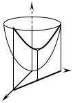
The function z = x2 + y 2 in fig. 1.13 has a relative |
Fig. 1.13 |
|
minimum when x= y = 0, which corresponds to a low |
|
|
point on the surface. In other words, the expression x2 + y 2 |
is positive number |
|
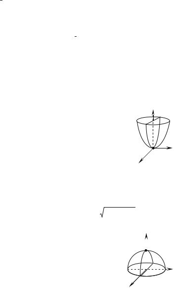
for any x and y and zmin = 0 at (0; 0). The change of z at (0; 0) is positive number: z(0;0) > 0 . Similarly, the function z = 4 − x2 − y 2 in fig. 1.14 has a
relative maximum at (0; 0) and zmax = 2 . The change of z |
z(0;0) < 0 . |
|
|
||
Let us look closely at the surface above a point |
z |
|
|
|
|
(x0, y0) where a relative maximum of f occurs. Assume |
|
|
|
||
2 |
|
|
|
||
that f is defined for all points within some circle |
|
|
|
||
|
|
|
|||
around (x0, y0) and possesses partial derivatives at (x0, |
|
|
|
|
|
y0). Let L1 be the line y = y0 in the xy plane; let L2 be |
|
|
|
|
|
the line x = x0 in the xy plane. (See fig. 1.15). Assume, |
О |
|
|
||
y |
|||||
for convenience, that the values of f are positive) |
|||||
2 |
|
|
|
||
Let C2 be the curve in the surface directly above |
x |
|
|
||
the line L1. Let C1 be the curve in the surface directly |
Fig. 1.14 |
|
|
||
above the line L2. Let M be the point on the surface directly above (x0, y0).
35
http://vk.com/studentu_tk, http://studentu.tk/
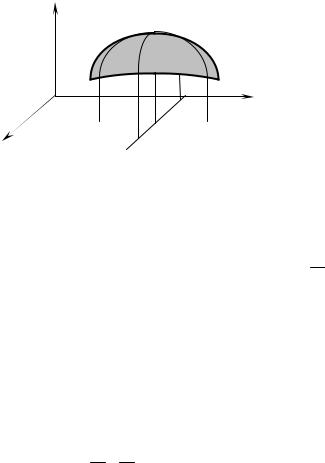
Since f has a relative maximum at (x0, y0), no point on the surface near M is higher than M. Thus M is the highest point on the curve C1 and on the curve C2 (for points near M). The study of functions of one variable showed that both these curves have horizontal tangents at M. In other words, at (x0, y0) both partial derivatives of f must be 0.
This conclusion is summarized in the following theorem.
zA relative maximum M
C1 C2 
|
|
|
y0 |
y |
|
x0 |
L2 |
||
x |
|
|
L1 |
|
|
|
|
||
|
|
|
|
|
|
|
|
Fig. 1.15 |
|
|
|
|
Let f be defined on a domain that includes the point |
|
Theorem 1 |
|
|
||
|
|
|
(x0, y0) and all points within some circle whose center is |
|
|
|
|
||
(x0, y0). If f has a relative maximum (or relative minimum) at (x0, y0) and ∂∂fx and
∂f |
exist at (x0, y0), then both these partial derivatives are 0 at (x0, y0); that is, |
|
||||
∂y |
f (x0 , y0 ) |
|
|
|
||
|
= 0, |
|
||||
|
|
|
|
|
||
|
|
x |
|
|||
|
|
|
|
|
|
|
|
|
f (x0 , y0 ) |
= 0. |
|
||
|
|
|
||||
|
|
|
y |
|
|
|
|
|
|
|
|
|
|
In other words, since |
|
|
|
|
|
|
|
dz(x0 , y0 ) = 0 . |
(1.11) |
||||
A point (x0, y0) for which ∂∂fx = ∂∂fy = 0 is called a critical point of f. Thus
from the theorem we infer that to locate relative extrema for a function we should examine its critical points.
The second-partial-derivative test for a relative maximum or minimum runs as follows.
36
http://vk.com/studentu_tk, http://studentu.tk/
|
|
|
|
|
|
|
|
|
Let |
|
M 0 (x0 , y0 ) |
be |
a |
|
critical |
point |
of the |
||||||||||||||||||||
|
|
|
Theorem 2 |
|
|
|
|
|
|
|
|||||||||||||||||||||||||||
|
|
|
|
|
|
|
|
|
|
|
|
|
function z = f (x, y) . Assume |
that the partial derivatives |
|||||||||||||||||||||||
|
|
|
|
|
|
|
|
|
|
|
|
|
|||||||||||||||||||||||||
∂f |
, |
|
∂f |
|
, |
∂ 2 f |
|
, |
|
∂ 2 |
f |
|
and |
|
∂ 2 |
f |
|
are continuous at and near M0. Let |
|
||||||||||||||||||
∂x |
|
∂y |
∂x2 |
|
∂x∂y |
|
|
∂y2 |
|
|
|||||||||||||||||||||||||||
|
|
|
|
|
|
|
|
|
|
|
|
|
|
|
|
|
|
|
|
|
|
|
|
|
|
||||||||||||
|
|
A = |
∂ 2 f (x |
0 |
, y |
0 |
) |
|
, |
B = |
∂ 2 |
f |
(x |
0 |
, |
y |
0 |
) |
, C = |
|
∂ 2 f (x |
0 |
, y |
0 |
) |
, |
= AC |
− B2 . |
|||||||||
|
|
|
∂x2 |
|
|
|
|
|
|
|
|
∂x∂y |
|
|
|
|
|
∂y 2 |
|
|
|
||||||||||||||||
|
|
|
|
|
|
|
|
|
|
|
|
|
|
|
|
|
|
|
|
|
|
|
|
|
|
|
|
||||||||||
Then
1)if > 0 , A > 0 ( C > 0) , then z has a relative minimum at M 0 (x0 , y0 ) ;
2)if > 0 , A < 0 ( C < 0) , then z has a relative maximum at M 0 (x0 , y0 ) ;
3)if < 0 , z has neither a relative maximum nor a relative minimum at
M 0 (x0 , y0 ) ;
4)if = 0 , no conclusion about extrema at M 0 (x0 , y0 ) can be drawn and
further analysis is required.
The quantity = AC − B2 is sometimes called the discriminant of z.
3.4. Relative extrema subject to the constraint
We shall now find relative maxima and minima for a function on which certain constraints are imposed.
Suppose we want to find the relative extrema of function z = f (x, y) subject to the constraint that x and y must satisfy
φ(x, y) = 0. |
( 1.12 ) |
It is any line L on the xy-plane. L contains a point M 0 (x0 , y0 ) .
|
A function |
z = f (M ) |
subject to the constraint has the relative extrema |
|||||||||||
|
at M 0 |
when x and y must satisfy (1.12 ), if a nearby point M 0 , exists such |
||||||||||||
|
that for any point M (x, y) ( M ≠ M 0 ) in this nearby on line L an inequality |
|||||||||||||
|
|
|
|
|
f (M ) > f (M 0 ) |
( f (M ) < f (M 0 ) )is provided |
|
|||||||
|
For example, the relative extrema of |
z = x2 + y 2 |
z |
|
||||||||||
subject to the constraint that |
x + y = 1 is at M 0 (1/ 2;1/ 2) |
|
|
|
||||||||||
|
|
|
||||||||||||
and the total relative extrema is at O(0; 0) |
(fig. 1.16 ). |
|
|
|
||||||||||
|
We can transform z, which is a function of two |
|
|
|
||||||||||
variables, into a function of one variable so that now the |
|
|
|
|||||||||||
function |
reflects |
constraint |
x + y = 1 . |
Solving this |
|
|
|
|||||||
equality for y, we get y = 1 − x , which when substituted |
О |
1 у |
||||||||||||
for y in z = x2 + y 2 gives |
|
|
|
|
х |
1 |
М0 |
|
||||||
|
|
z = x |
2 |
+ (1 − x) |
2 |
= |
2x |
2 |
− 2x + 1 . |
|
|
|||
|
|
|
|
|
|
Fig. 1.16 |
||||||||
|
|
|
|
|
|
|
|
|
|
37 |
|
|
|
|
http://vk.com/studentu_tk, http://studentu.tk/

Since z is now expressed as a function of one variable, to find relative extrema we follow the usual procedure of setting its derivative equal to 0:
z′ = 4x − 2 = 0 x = 12 and z′′ = 4 > 0 .
Thus z, subject to the constraint, has a relative minimum at M 0 (1/ 2;1/ 2)
and zmin = 12 .
Let x = x(t) , y = y(t) describe a subject parametrically, in other words, since ϕ(x(t), y(t)) ≡ 0 ,
to find relative extrema of a function of one variable z = f (x(t), y(t)) .
Often this is not practical, but there is another technique, called the method of Lagrange multipliers, that avoids this step and yet allows us to obtain critical points.
The method is as follows. Suppose we have a function z = f (x, y) subject to the constraint ϕ(x, y) = 0 . We construct a new function L of three variables defined by the following:
L(x, y, λ) = f (x, y) + λϕ(x, y) . |
(1.13 ) |
|
|
It can be shown that if M 0 (x0 , y0 ) is a critical point of z subject to the constraint ϕ(x, y) = 0 , there exists a value of λ, say λ0, such that (x0, y0, λ0) is a
critical point of z. The number λ0 is called a Lagrange multiplier. Also, if (x0, y0, λ0) is a critical points of z, then (x0, y0) is a critical point of z subject to the constant. Thus to find critical of z subject to ϕ(x, y) = 0 , we instead find critical points of
z. They are obtained by solving the simultaneous equations.
∂L = 0,
∂x
∂L = 0, (1.14)
∂x
ϕ(x, y) = 0.
At times, ingenuity must be used to do this. Once we obtain a critical point (x0, y0, λ0) of f we can conclude that M0(x0, y0) is a critical point of f subject to the constraint ϕ(x, y) = 0 . Although f and ϕ are functions of two variables, the
method of Lagrange multipliers can be extended to n variables.
Finally, if is defined the sign of the second-order deferential d 2 L of the Lagrange function condition under such circumstances:
dϕ = 0 ∂∂ϕx dx + ∂∂ϕy dy = 0 . 38
http://vk.com/studentu_tk, http://studentu.tk/

If d 2 L(M0 ) > 0 , then z, subject to constraint, has a relative minimum at M 0 . If d 2 L(M0 ) < 0 , then z, subject to constraint, has a relative maximum at M 0
3.5. Extrema on a polygon
If D consists of the region bounded by a polygon including its boundary and z = f (x, y) is continuous throughout D, then z has a maximum value at some
point in D. This situation is similar to the maximum-value theorem, which concerns a continuous function defined on a closed interval [a, b]. Proofs of both results are to be found in any advanced calculus text. The theorem also holds if D is bounded by a curve. (D is also assumed to be “finite” in the sense that it lies within some circle.) A similar result holds for the minimum value of z on D.
The procedure is similar to that for maximizing (minimizing) a function on a closed interval:
1. First find any points that are in D but not on the boundary of D where both
∂∂xz and ∂∂yz are 0. These are called critical points. (If there are no critical points,
the maximum or minimum occurs on the boundary.)
2. If there are critical points, evaluate z at them. Also find the maximum (minimum) of z on the boundary. The maximum (minimum) of z on D is the largest (smallest) value of z on the boundary and at critical points.
|
Т.3 |
|
|
|
Typical problems |
|
|
|
|
|
|
|
|
|||||||||||
1. Find the equations of the |
tangent |
plane and |
normal line to a surface |
|||||||||||||||||||||
z = x 2 y + xy3 |
at point (2, 1). |
|
|
|
|
|
|
|
|
= 22 1 + 2 13 = 6. |
||||||||||||||
Solution. We have |
|
x0 |
= 2 , |
y0 = 1. First compute z0 |
||||||||||||||||||||
Evaluating |
∂z |
and |
∂z |
|
at (2, 1): |
|
|
|
|
|
|
|
|
|
||||||||||
∂x |
∂y |
|
|
|
|
|
|
|
|
|
||||||||||||||
|
|
|
|
|
|
|
|
|
|
|
|
|
|
|
|
|
|
|
|
|||||
|
|
∂z |
|
= |
2xy + y |
3 |
, |
|
∂z |
|
= x |
2 |
+ 3xy |
2 |
; |
∂z(2;1) |
= |
5 ; |
∂z(2;1) |
=10 . |
||||
|
|
∂x |
|
|
|
|
∂y |
|
|
∂x |
|
∂y |
||||||||||||
|
|
|
|
|
|
|
|
|
|
|
|
|
|
|
|
|
|
|
||||||
By the table lists 1.1 and 1.2 we have an equation of the tangent plane z − 6 = 5(x − 2) + 10( y − 1) , or 5x + 10 y − z − 14 = 0 ,
and an equation of the normal line
x − 2 = y − 1 = z − 6 . 5 10 − 1
2. Find the equations of the tangent plane and normal line to a surface x3 + y3 + z3 + xy2 z3 = 4
at point M 0 (1; 1; 1) .
39
http://vk.com/studentu_tk, http://studentu.tk/
Solution. By the table lists 1.1 and 1.2 we have
|
|
|
F = x3 + y3 + z3 + xy 2 z |
3 − 4 ; |
|
∂F |
= 3x2 + y 2 z3 , |
|
|
|
|
||||||||||||||||||||||||||||||
|
|
|
|
∂x |
|
|
|
|
|||||||||||||||||||||||||||||||||
|
|
|
|
|
|
|
|
|
|
|
|
|
|
|
|
|
|
|
|
|
|
|
|
|
|
|
|
|
|
|
|
|
|
|
|
|
|
||||
|
|
|
|
|
∂F |
= 3y 2 + 2xyz3 ; |
∂F |
= 3z 2 + 3xy2 z 2 ; |
|
|
|
|
|||||||||||||||||||||||||||||
|
|
|
|
|
∂y |
|
|
|
|
|
|
|
|
|
|
∂z |
|
|
|
|
|
|
|
|
|
|
|
|
|
|
|
|
|
|
|
|
|
||||
|
|
|
|
|
∂F(M 0 ) |
= 4 ; |
|
∂F(M |
0 ) |
|
|
= 5 |
; |
|
|
∂F(M 0 ) |
= 6 . |
|
|
|
|
|
|
|
|||||||||||||||||
|
|
|
|
|
|
∂x |
|
|
|
|
|
∂y |
|
|
|
|
|
|
|
∂z |
|
|
|
|
|
|
|
|
|||||||||||||
|
|
|
|
|
|
|
|
|
|
|
|
|
|
|
|
|
|
|
|
|
|
|
|
|
|
|
|
|
|
|
|
|
|
|
|
||||||
An equation of the tangent plane is |
|
|
|
|
|
|
|
|
|
|
|
|
|
|
|
|
|
|
|
|
|
|
|
|
|
|
|||||||||||||||
|
4(x − 1) + 5( y − 1) + 6(z −1) = 0 , or 4x + 5y + 6z − 15 = 0 , |
|
|
|
|||||||||||||||||||||||||||||||||||||
and an equation of the normal line is |
|
y −1 |
|
|
|
|
|
|
|
|
|
|
|
|
|
|
|
|
|
|
|
|
|
|
|
|
|||||||||||||||
|
|
|
|
|
|
|
|
|
x − 1 |
= |
|
= |
z −1 |
. |
|
|
|
|
|
|
|
|
|
|
|
|
|||||||||||||||
|
|
|
|
|
|
|
|
|
|
|
|
|
|
|
|
|
|
|
|
|
|
|
|
|
|
|
|
|
|||||||||||||
|
|
|
|
|
|
|
|
4 |
|
|
|
|
|
|
5 |
|
|
|
|
|
6 |
|
|
|
|
|
|
|
|
|
|
|
|
|
|
|
|
||||
3. |
Calculate the |
derivative |
|
of |
a function u = x2 y + xy 2 z + z3 |
at |
point |
||||||||||||||||||||||||||||||||||
M (0;1; − 1) |
in the direction of the vector l =−2i + j +2k . |
|
|
|
|
||||||||||||||||||||||||||||||||||||
Solution. We find the directional cosines of the vector l |
: |
|
|
|
|
|
|
|
|||||||||||||||||||||||||||||||||
l ={−2, 1, 2}, | l |= 4 +1+4 = 3 , |
|
cos α = − |
2 |
, cos β = |
1 |
, cos γ = |
2 |
. |
|||||||||||||||||||||||||||||||||
|
3 |
|
3 |
||||||||||||||||||||||||||||||||||||||
|
|
|
|
|
|
|
|
|
|
|
|
|
|
|
|
|
|
|
|
|
|
|
|
|
|
|
|
|
|
|
|
|
3 |
|
|
|
|||||
Then we calculate the partial derivatives of a given function at M (0;1;−1) : |
|||||||||||||||||||||||||||||||||||||||||
|
|
|
∂u(M ) = 2xy + y 2 z |
|
M = −1 ; |
|
∂u(M ) |
= x2 + 2xyz |
|
M = 0 ; |
|
|
|
||||||||||||||||||||||||||||
|
|
|
|
|
|
|
|
||||||||||||||||||||||||||||||||||
|
|
|
∂x |
|
∂u(M ) |
|
|
|
|
|
|
|
|
|
|
|
∂y |
|
|
|
|
|
|
|
|
|
|
|
|
|
|||||||||||
|
|
|
|
|
|
|
|
= xy2 |
+ 3z 2 |
|
M = 3 . |
|
|
|
|
|
|
|
|
|
|
|
|||||||||||||||||||
|
|
|
|
|
|
|
|
|
|
|
|
|
|
|
|
|
|
|
|
||||||||||||||||||||||
Then, by (2.10), |
|
∂u |
∂z |
|
|
|
|
|
2 |
|
|
|
|
1 |
|
|
|
|
2 |
|
8 |
|
|
|
|
|
|
|
|
|
|||||||||||
|
|
|
|
|
|
|
|
|
|
|
|
|
|
|
|
|
|
|
|
|
|
|
|
|
|||||||||||||||||
|
|
|
|
|
|
|
|
|
|
|
|
|
|
|
|
|
|
|
|
|
|
|
|
|
|
|
|
|
|
|
|||||||||||
|
|
|
|
|
|
|
∂l |
= (−1) |
− |
|
+ 0 |
|
|
|
+ |
3 |
|
= |
|
|
. |
|
|
|
|
|
|
|
|||||||||||||
|
|
|
|
|
|
|
3 |
3 |
3 |
3 |
|
|
|
|
|
|
|
|
|||||||||||||||||||||||
|
|
|
∂u |
|
|
|
|
|
|
|
|
|
|
|
|
|
|
|
|
|
|
|
|
|
|
|
|
|
|
|
|
|
|||||||||
We have |
|
> 0 , hence the function u(x, y, z) |
at point М in the direction of |
||||||||||||||||||||||||||||||||||||||
|
|
||||||||||||||||||||||||||||||||||||||||
|
|
|
∂l |
|
|
|
|
|
|
|
|
|
|
|
|
|
|
|
|
|
|
|
|
|
|
|
|
|
|
|
|
|
|
|
|
|
|
|
|
||
the vector l |
is decreasing. |
|
|
|
|
|
|
|
|
|
|
|
|
|
|
|
|
|
|
|
|
|
|
|
|
|
|
|
|
|
|
|
|
|
|
||||||
4. |
Find |
an angle |
between the |
gradients |
|
of |
function |
u = |
xy |
at points |
|||||||||||||||||||||||||||||||
M1 (2; |
2; 1) |
and M2 |
(1; 1; −1) . |
|
|
|
|
|
|
|
|
|
|
|
|
|
|
|
|
|
|
|
|
|
|
|
|
|
|
|
z |
|
|
|
|||||||
|
|
|
|
|
|
|
|
|
|
|
|
|
|
|
|
|
|
|
|
|
|
|
|
|
|
|
|
|
|
|
|||||||||||
Solution. We find an angle between the vectors a1 and a2 by the formula |
|||||||||||||||||||||||||||||||||||||||||
|
|
|
|
|
|
|
|
|
cos ϕ = |
a1a2 |
|
|
|
. |
|
|
|
|
|
|
|
|
|
|
|
|
|
|
|||||||||||||
|
|
|
|
|
|
|
|
|
| a |
|| a |
| |
|
|
|
|
|
|
|
|
|
|
|
|
|
|
|
|||||||||||||||
|
|
|
|
|
|
|
|
|
|
|
|
|
|
|
|
|
|
|
|
|
|
|
|
|
|
|
|
|
|
|
|
|
|
||||||||
|
|
|
|
|
|
|
|
|
|
|
|
|
|
|
|
|
1 |
2 |
|
|
|
|
|
|
|
|
|
|
|
|
|
|
|
|
|
|
|
||||
|
|
|
|
|
|
|
|
|
|
|
|
|
|
|
|
40 |
|
|
|
|
|
|
|
|
|
|
|
|
|
|
|
|
|
|
|
|
|
|
|
|
|
http://vk.com/studentu_tk, http://studentu.tk/