

Higher_Mathematics_Part_2
.pdfKyiv
National Aviation University
«NAU-druk » Publishing
2009
http://vk.com/studentu_tk, http://studentu.tk/
UDC 51(075.8)
ББК В11я7
Н 65
All rights reserved. No part of this book may be reproduced in any form without the prior written permission of the publisher
Reviewers:
O. P. Besklinska — candidate of science (physics and mathematics), associate professor
(Kyiv National Linguistic University)
P.T. Kachanov — candidate of science (engineering), associate professor (State University of Information and Communication Technologies)
English language adviser
O. M. Akmaldinova — (philology) professor
Approved by the Methodical and Editorial board of the National Aviation University (Minutes № 7/09 of 01.07.2009)
The manual fully corresponds to the educational program of higher mathematics for engineering universities. It contains basic theoretical information, examples of problems solution, class, home and self-test assignments.
The manual is intended for the first year students of all specialties
ISBN 978-966-598-316-4 |
© V. P. Denisiuk, V. G. Demydko, |
V. K. Repeta, 2009 |
|
ISBN 978-966-598-476-4 |
© NAU, 2009 |
http://vk.com/studentu_tk, http://studentu.tk/

CONNTENTS
INTRODUCTION................................................................................................ |
4 |
Module 1 |
|
FUNCTIONS OF SEVERAL VARIABLES AND COMPLEX NUMBERS ..... |
5 |
Topic 1. |
|
Functions of several variables. Limits, and continuous functions .................. |
5 |
Topic 2. |
|
Partial derivatives and differentials of a function of several variables ......... |
15 |
Topic 3. |
|
Applications of partial derivatives................................................................ |
33 |
Topic 4. |
|
Complex numbers......................................................................................... |
52 |
Module 2 |
|
INTEGRAL CALCULUS.................................................................................. |
63 |
Topic 1. |
|
Indefinite integral ......................................................................................... |
63 |
Topic 2. |
|
Polynomials. The rational functions ............................................................. |
88 |
Topic 3. |
|
Integration of rational functions by partial fractions .................................... |
99 |
Topic 4. |
|
Integrals involving powers of trigonometric functions............................... |
114 |
Topic 5. |
|
Integration of irrational functions............................................................... |
128 |
Topic 6. |
|
Definite integrals ........................................................................................ |
144 |
Topic 7. |
|
Improper integrals....................................................................................... |
155 |
Topic 8. |
|
Application of the definite integral............................................................. |
164 |
Module 3 |
|
DIFFERENTIAL EQUATIONS...................................................................... |
184 |
Topic 1. |
|
Differential equations of the first order and the first degree....................... |
184 |
Topic 2. |
|
Differential equations of order higher than the first ................................... |
205 |
Topic 3. |
|
Linear differential equation with constant coefficient ................................ |
212 |
Topic 4. |
|
Simultaneous differential equations............................................................ |
230 |
LITERATURE ................................................................................................. |
242 |
3
http://vk.com/studentu_tk, http://studentu.tk/

INTRODUCTION
This book offers the modular technology of studying higher mathematics course by the students of engineering specialties in the first term.
The module represents the logically compiled sections of studied subject.
The material of the first term is divided into three modules: 1. Functions of several variables and complex numbers.
2.Integral calculus.
3.Differential equations. The module contains several.
Every module begins with the general statements, which represent the
themes of the sections, basic concepts, and main tasks. The micromodule covers:
1)basic theoretical information,
2)examples of problem solutions,
3)class and home assignments,
4)self-test assignments.
The theoretical part gives all necessary material for mastering the theme in question (lecture summary). The references to the literature are applied to all the themes, which enable the students to master their theoretical material.
The practical part contains examples of problem solutions, that illustrate the theoretical material and problems with answers for class and home work.
Each micromodule is provided with self-test assignments which contain several problems to be done by the students in a written form.
4
http://vk.com/studentu_tk, http://studentu.tk/

Module
FUNCTIONS OF SEVERAL VARIABLES AND COMPLEX NUMBERS
Objective. This chapter develops the concepts of the multivariable calculus and the complex numbers. The topics will be used to learn the other topics of high mathematics and natural sciences.
Structure of the module
Topic 1. Functions of several variables. Limits and continuous functions.
Topic 2. Partial derivatives and a differential of the functions of several variables.
Topic 3. Applications of partial derivatives.
Topic 4. Complex numbers. Forms of the complex numbers. Operations with them
Basic concepts. 1. Functions of several variables. 2. Limit, and continuity of the functions of several variables. 3. Partial derivatives. 4. Differential. 5. Relative extrema. 6. Tangent plane and normal to a surface. 7. Gradient.
8.Complex number. 9. Module and argument of a complex number. Basic problems. 1. Finding domain of a function of several variables.
2.Finding the first and higher order partial derivatives and the differentials.
3.Finding partial derivatives of the composite functions. 4. Implicit partial
differentiation. 5. Finding relative extrema and extrema on a polygon. 6. Operations with complex numbers.
Topic 1. Functions of several variables. Limits and continuous functions
Concepts of a function of several variables. Limit functions of several variables. Continuous functions of two variables.
Literature: [2, section 1, § 1.1], [3, ch. 6, § 1], [6, section 6, § 6.1.], [7, section 8, §§1—4], [9, § 43].
5
http://vk.com/studentu_tk, http://studentu.tk/
|
Main concepts |
Т.1 |
1.1. Definitions
Let D be the given region consisting of ordered pairs of real numbers (x,y). Function z is defined as a function of x and y is called a function of two variables and denoted by z = f(x, y).
The variable z is called a dependent value (function), x and y — are called independent values (arguments).
The domain of z = f(x, y) is all ordered pairs of real numbers (x,y) for which the equation has the meaning when the first and second elements of (x,y) are substituted for x and y, respectively, in the equation and denoted D(f) or D.
The region consisting of plurality of z is denoted E(f) or E.
We can represent geometrically a function of two variables, z = f(x, y). To each ordered pair (x, y) in the domain of the function f we assign point M(x, y) in the x, y-plane. So, you can consider z = f(x, y) as function of point M(x, y) and write z = f(M).
Quantity of function z = f (x, y) in point M0 (x0, y0) is denoted by z0 = f (x0,
y0), or z0 = f (M0), or z = z |
M 0 . |
|
|
To |
each |
point P in |
space we |
can |
||||
z |
|
|
|
|
||||||||
|
|
|
assign a unique ordered triple of |
|||||||||
|
|
|
|
|||||||||
z0 |
|
|
|
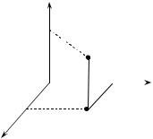
numbers, called the coordinate of P. To |
||||||||
|
|
|
do |
this (see |
fig. 1.1), |
from |
P |
we |
||||
|
|
|
|
|||||||||
|
P(x0, y0, z0) |
|
construct a line perpendicular to the x, |
|||||||||
|
|
y-plane, that is, the plane determined by |
||||||||||
|
|
|
|
|||||||||
O |
y0 |
y |
the x- and y- axes. Let M be the point |
|||||||||
where |
the |
line |
intersects this |
plane. |
||||||||
x0 |
M |
|
From M we construct perpendiculars to |
|||||||||
|
the |
x- |
and |
y-axis at |
x0 and |
y0 |
||||||
x |
|
|
|
|||||||||
Fig. 1.1 |
|
respectively. From P a perpendicular to |
||||||||||
|
|
|||||||||||
|
|
the |
z-axis |
|
is |
constructed |
which |
|||||
|
|
|
|
|
||||||||
intersects it at z0. Thus to P we assign the ordered triple (x0, y0, z0). It should also be evident that with each ordered triple of numbers we can assign a unique point in space. Due to this one-to-one correspondence between points in space and ordered triples, an ordered triple may be called a point.
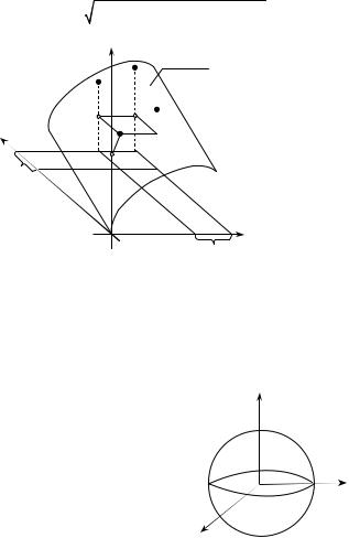
The function of two variables, z = f (x, y), its domain (consisting of ordered pairs of real numbers) can be geometrically represented by a region in the xy-plane. The graph of z = f (x, y) is a surface (see fig. 1.2).
In general, a function of m variables is one whose domain consists of ordered m –– tuples ( x1 , x2 , ..., xm ). Although functions of several variables are extremely impotent and useful, we cannot represent geometrically functions of
6
http://vk.com/studentu_tk, http://studentu.tk/
more than two variables. However we can consider ( x1 , x2 , ..., xm )as the coordinates of a point of ordered m –– tuples. It is denoted by M(x1, x2, …, xm,).
The distance between two points M(x |
|
, x , …, x |
m |
,) and |
M |
0 |
(x0; |
x0; |
…; x0 ) is |
||||||||
defined by the formula |
|
1 |
2 |
|
|
|
|
|
|
1 |
2 |
|
m |
||||
|
|
|
|
|
|
|
|
|
|
|
|
|
|
|
|
|
|
ρ(M , M |
0 |
) = (x −x0 )2 |
+…+(x −x0 |
|
)2 . |
|
|
|
|||||||||
|
1 |
1 |
|
|
|
|
m |
m |
|
|
|
|
|
|
|||
|
|
z |
|
|
z = f(x, y) |
|
|
|
|
|
|
|
|
||||
|
|
|
|
|
|
|
|
|
|
|
|
|
|||||
|
|
z |
|
|
|
|
|
|
|
|
|
|
|
|
|
|
|
|
|
zy |
|
|
|
|
|
|
|
|
|
|
|
|
|
|
|
y |
|
|
|
|
zx |
|
|
|
|
|
|
|
|
|
|
|
|
|
(x,y,f(x,y)) |
|
|
|
|
|
|
|
|
|
|
|
|||||
y y |
|
f(x,y) |
|
|
|
|
|
|
|
|
|
|
|
|
|
|
|
|
|
|
|
|
|
|
|
|
|
|
|
|
|
|
|
|
|
|
|
Fig. 1.2 |
|
|
|
x |
|
x |
x |
|
|
|
|
|
|
|
|
|
|
|
|
|
|
|
|
|
|
|
|
|
|
|
|
|
|
The set of all points |
Мi, the coordinates of |
each |
|
assign |
an |
inequality |
|||||||||||
ρ(M , M 0 ) < ε , is called the nearby of point |
M 0 . For instance the nearby of |
||||||||||||||||
point M0 (x0 , y0 ) is the set all inside points of a circle with radius is ε and |
|||||||||||||||||
center in M0. |
|
|
|
|
|
|
|
|
|
|
|
|
|
|
|
|
|
If a line bounds the region D it is called |
|
|
|
|
z |
|
|
|
|
|
|
||||||
the range of the domain D. The points in |
|
|
|
|
|
|
|
|
|
|
|||||||
|
|
|
|
|
|
|
|
|
|
|
|
||||||
the domain but not on the range are called |
|
|
|
|
2 |
|
|
|
|
|
|||||||
inside points. This domain is called the |
|
|
|
|
|
|
|
|
|
||||||||
|
|
|
|
|
|
|
|
|
|
|
|
||||||
close domain. The domain involving the |
|
|
|
|
|
|
|
|
|
|
|
|
|||||
points inside the range and on it boundary is |
|
|
|
|
O |
|
|
|
|
|
|||||||
called the open domain. |
|
|
|
|
|
|
|
|
|
|
|
|
2 |
y |
|||
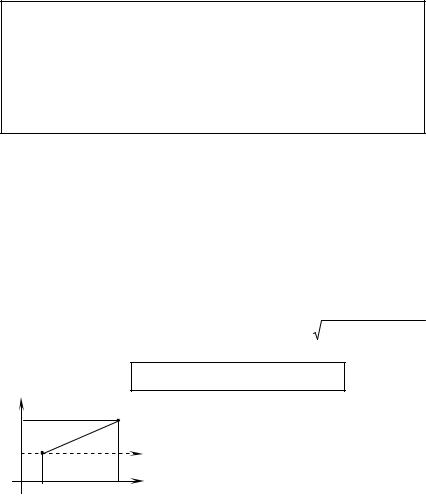
The domain of a function |
|
|
|
|
|
|
|
|
|
|
|
|
|
||||
|
|
|
|
|
|
|
|
|
|
|
|
|
|
|
|||
u = ln(4 – x2 – y2 – z2) |
|
|
|
|
|
x |
|
|
|
|
|
|
|
|
|
|
|
is the set of all points inside a sphere |
of |
|
|
Fig. 1.3 |
|
|
|
||||||||||
|
|
|
|
|
|
|
|||||||||||
radius 2 and center (0,0,0). The graph is |
|
|
|
|
|
|
|
||||||||||
|
|
|
|
|
|
|
|
|
|
|
|
||||||
shown in fig. 1.3. |
|
|
|
|
|
|
|
|
|
|
|
|
|
|
|
|
|
The boundary of the sphere is not in the domain u. The range in this problem is the interval (–∞; ln 4).
7
http://vk.com/studentu_tk, http://studentu.tk/
1.2. Limit of a function of two variables
Let z = f(x, y) be the function in the domain D and a point M0 on the range D, which may be or may not be in the domain D, that is M0 D or M0 D .
Let’s assume that domain D contains one or some points a nearby M0. Whether a function has a limit is independent of the ways of approache to the
point. The limit of the function of several variables does not exist if some ways of point M approaches to M0 occur.
Let f be a function of two variables and b some fixed number. Number b is called the limit of function f(M) at a point M(x0, y0) if for any ε > 0 there exist number δ > 0 that for all points M(x, y) such meating the condition 0 <ρ (M, M0) < δ, the following inequalty
|
f (x, y) − b |
|
< ε |
lim f (M ) = b |
|
|
|||
occurs and is denoted as lim f (x, y) = b or |
||||
x→ x0 , |
M →M0 |
|||
y→ y0 |
|
|||
Evaluating the limits is accomplished in the following steps.
1. Change origin in to point M0 (x0 , y0 ) . For instance if x ≠ x0, use a substitution
x − x0 , if x0 ≠ 0, x0 ≠ ∞, |
|
|
|||||
|
1 |
|
|
|
|
|
|
t = |
, |
if |
x0 = ∞. |
|
|
||
|
|
|
|
||||
x |
|
|
|||||
|
|
|
|
1 |
|
||
For example if M (x; y) → M0 |
(2; |
∞) |
use substitutions t1 = x – 2, t2 = |
. |
|||
|
|||||||
|
|
|
|
|
y |
||
Thus M (t1 , t2 ) → M0 (0; 0) .
2. Sometimes polar coordinates are used. If M0(x0,y0) is a pole and the positive X-axis is the polar axis (fig. 1.4), a point with a polar representation (ρ, ϕ)
has a rectangular representation (x, y), where and ρ = (x − x0 )2 + (y − y0 )2 ,
0 ≤ ρ ≤ ∞, 0 ≤ ϕ ≤ 2π.
x – x0 = ρ cosϕ, y – y0 = ρ sinϕ.
Y
у
ρ
y0 M0 φ
Оx0
Fig. 1.4
M |
Thus, finding |
lim |
f (M ) |
is calculated |
to lim f (M ) , where |
M →M0 |
|
||
|
ρ is |
one of |
coordinates of |
|
|
ρ→0 |
|
|
|
p |
point М, the second |
coordinate is any angle ϕ. |
||
|
Note that the limit exist |
if and only if the limit |
||
х Х |
exists with ρ → 0 for any dependences ϕ = ϕ (ρ) |
|||
|
and θ = θ(ρ). |
|
|
|
|
8 |
|
|
|
http://vk.com/studentu_tk, http://studentu.tk/

1.3. Continuous functions of two variables
Let’s assume that u = f(x, y) is defined at M 0 (x0 ; y0 ) . Then the function f is continuous at M0 if
|
lim f (x, y) = f (x0 , y0 ) , |
(1.1) |
|||
|
x→ x |
0 , |
|
|
|
|
y→ y0 |
|
|||
that is |
|
|
|
|
|
|
|
lim f(M) = f(M0) |
|
|
|
|
|
|
|
|
|
|
|
M →M0 |
|
|
|
Note, thet point М approache M 0 by any way in the domain of u. |
|
||||
Let x − x0 = |
x , y − y0 = |
y . Then formula (1.1) can be represented as |
|||
|
lim [ f (x, y) − f (x0 , y0 )] = 0 or lim u = 0 , |
|
|||
|
x→0, |
|
ρ→0 |
|
|
|
y→0 |
|
|
|
|
where Δρ = ( |
x)2 + ( y)2 |
is the distance between М and M 0 , |
u is the |
||
change of function u at point M0.
Then f is a continuous function if it is continuous at each point in its domain. The function has a discontinuety at point M0 if the following cases occur:
1) function is defined at all points nearby M0 except M0;
2) function is defined at M0 and nearby it, but |
lim |
f (M ) does not exist; |
||
|
|
|
M →M 0 |
|
3) function is defined at all points nearby of M0 and |
lim f (M ) exists, but |
|||
lim f (M ) ≠ f (M 0 ) . |
M →M 0 |
|||
|
|
|||
M →M 0 |
|
|
|
|
|
Properties of the continuous functions of two variables |
|||
|
|
in the close and bounded region |
|
|
|
|
Assume that z = f (x, y) |
is a continuous function in the |
|
|
Theorem 1 |
|||
|
close region D. Then the function |
is bounded in D and |
||
|
|
|||
moreover a number M > 0 exists, such that for all points of region D inequality | f (x, y) |< M occurs.
|
|
Assume that z = f (x, y) |
is a continuous function in the |
|
Theorem 2 |
||
|
close region D. There are the points in it, where the |
||
|
|
|
|
function has the minimum and maximum values. |
|
||
|
|
Assume that z = f (x, y) |
is a continuous function in the |
|
Theorem 3 |
||
|
close region D. Then the function is bounded in D and |
||
|
|
||
moreover there are the points M1 and M2 in it, where the function has the values with the diverse signs. Hence f(M1) f(M2) < 0. A point M0 D exists where f(M0) = 0.
9
http://vk.com/studentu_tk, http://studentu.tk/
Т.1 |
Typical problems |
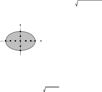
1. Determine the domain of the function z = 36−4x2 −9y2 .
Solution. The domain is the set of all real numbers z(x, y) such that the
radicand 36 – 4x2 – 9y2 is nonnegative. So, 36 − 4x2 − 9y 2 ≥ 0 . |
|
|||||||||||||||||||||
|
|
y |
|
|
|
|
|
|
The |
|
range of the |
domain is |
an ellipse |
|||||||||
|
|
|
|
4x 2 + 9 y 2 = 36 |
|
or |
|
in |
standard |
position |
||||||||||||
2 |
|
|
|
x |
2 |
|
+ |
y |
2 |
= 1. It |
has |
a |
center at origin and x |
|||||||||
|
|
|
|
|
|
|
|
|
||||||||||||||
|
|
|
|
|
9 |
|
|
|
||||||||||||||
|
–3 |
3 x |
|
|
|
4 |
|
|
|
|
|
|
|
|
|
|||||||
|
intercepts are 3 and –3; y intercepts are 2 and |
|||||||||||||||||||||
|
|
|
|
|
–2. The graph is shown in fig. 1.5. The set of |
|||||||||||||||||
|
|
|
|
|
all points inside an ellipse and on the range of |
|||||||||||||||||
|
|
–2 |
|
|
ellipse are domain of z. For instance, the point |
|||||||||||||||||
|
|
|
|
(0, 0) is inside the ellipse because is occur the |
||||||||||||||||||
|
|
|
|
|
||||||||||||||||||
|
|
Fig. 1.5 |
|
|
inequality 36 – 4 0 – 9 0 > 0. A point (3, 0) is |
|||||||||||||||||
36 – 4 32 – 9 0 = 0 occur. |
|
on the range of the ellipse because the equality |
||||||||||||||||||||
|
|
|
|
|
|
|
|
|
|
|
|
|
|
|
|
|
|
|
||||
|
The range of z(x, y) is [0, 6] . |
|
|
|
|
|
|
|
|
|
|
|
|
|
|
|
|
|||||
|
2. Determine the domain of the function |
|
|
|
|
|
|
|
|
|||||||||||||
|
|
|
z = |
y − x + |
2 + arcsin |
x2 |
+ y2 |
. |
|
|
|
|||||||||||
|
|
|
|
|
4 |
|
|
|
|
|||||||||||||
|
|
|
|
|
|
|
|
|
|
|
|
|
|
|
|
|
|
|
|
|
|
|
|
|
Solution. The are two factors acting on the domain |
|
|
|
|
||||||||||||||||
|
|
|
y − x + 2 ≥ 0, |
|
|
|
|
y ≥ x − 2, |
|
|
||||||||||||
|
|
|
|
|
x2 + y |
|
|
|
|
|
|
or |
|
|
|
|
||||||
|
|
|
|
−1 ≤ |
2 |
|
≤ 1, |
|
|
2 |
|
2 |
|
|
|
|||||||
|
|
|
|
|
|
|
|
|
|
|
|
x |
|
+ y |
|
≤ 4. |
|
|
||||
|
|
|
|
|
4 |
|
|
|
|
|
|
|
|
|
|
|
|
|
||||
|
|
|
|
|
|
|
|
|
|
|
|
|
|
|
|
|
|
|
|
|
||
|
The inequality |
y ≥ x − 2 |
is the |
|
upper |
half-plane of |
the straight line |
|||||||||||||||
y = x + 2 , including it. The inequality |
|
x2 + y 2 ≤ 4 is a circle with the center at |
||||||||||||||||||||
the origin and radius two. The intersection of these regions is the domain D of z (fig. 1.6).
3. Calculate lim (x2 + y2 ) arctg |
x |
. |
|
|
|
|
|
|
|
||||
|
|
|
|
|
|
|
|
||||||
x→0, |
|
|
|
y |
|
|
|
|
|
|
|
||
y→0 |
|
|
|
|
|
|
|
|
|
|
|
|
|
Solution. A function |
arctg |
x |
is bounded: |
− |
π |
< arctg |
x |
< |
π |
. |
|||
y |
2 |
y |
2 |
||||||||||
|
|
|
|
|
|
|
|
|
|||||
If x → 0 and y → 0 the sum |
x2 + y 2 is an infinitely less value. The product |
||||||||||||
of bounded and infinitely less values is an infinitely less value:
10
http://vk.com/studentu_tk, http://studentu.tk/