Ohrimenko+ / Barnsley. Superfractals

Table 4.3 A projective IFS code. This is used in Figure 4.4

Table 4.4 Affine IFS code for a filled square. The IFS is strictly contractive, but not with respect to the usual euclidean metric. This is an example of an overlapping IFS

An example of an affine hyperbolic IFS is

F1 = R2; 12 x, 12 y , 12 (x + 1), 12 y , 12 x, 12 (y + 1) .

Here the transformations are defined by their actions on the point (x, y) R2. We identify them by the labels 1, 2 and 3, as in f1, f2 and f3 respectively.

Notice that although the space (R2, deuclidean ) is not compact, closed bounded subsets of it are. It is straightforward to show that there exists a compact subset X of R2 such that fn : X → X for n = 1, 2, . . . , N . See Exercise 4.4.1.

The IFS F1 may be specified succinctly by means of the array in Table 4.2, which we refer to as an affine IFS code. The affine transformations are denoted

Table 4.6 Example of a Mobius¨ IFS code

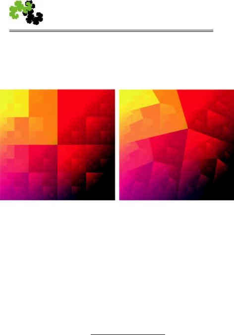
Figure 4.4 This illustates IFS colouring applied to two different IFSs with the same attractor; see the main text. It is suggestive of a homeomorphism between the two pictures. But the fractal dimensions of the level sets may not be the same.

Notice that an affine IFS can be represented by a projective IFS code in which g = h = 0 and j = 1.

where = {z C : |z| ≤ 1}. This IFS may be represented by the Mobius¨ IFS code in Table 4.6, where the coefficients reference transformations written in the form

f (z) = (aR + iaI )z + (bR + ibI ) . (cR + icI )z + (dR + idI )

Note that when the transformations of an IFS belong to a particular geometry then so do their attractors, in the sense described in Section 3.7.

E x e r c i s e 4.4.1 Let F be a hyperbolic IFS. Show that there exists a closed ball of finite radius in X that is mapped into itself by the transformations of the IFS. Show therefore that if X is a locally compact metric space then there exists X such that {X; f1, f2, . . . , fN } is a hyperbolic IFS, where X is compact.

E x e r c i s e 4.4.2 Prove that all three transformations referenced in Table 4.4 are strictly contractive with respect to the metric

d((x1, y1), (x2, y2)) = (x1 − x2)2 + 14 (y1 − y2)2.

Find two points that are not moved closer together, in the euclidean metric, by the third transformation.

4.5 The chaos game

The ‘chaos game’ is our name for a well-known type of algorithm, namely the Markov Chain Monte Carlo (MCMC) or random iteration algorithm. The scholarly history of the chaos game is discussed in [91] and in [55] and it appears that it began in 1935 with the work of Onicescu and Mihok, [76]. Its usage in computing approximations to the invariant probability measure and the set attractor of a hyperbolic IFS is justified by the following theorem, which can be proved with the aid of Birkhoff’s ergodic theorem; see for example [39]. See also [22], and [28]. It was introduced to fractal geometry in [64] and [4]; see also [7].

T h e o r e m 4.5.1 Let (X, d) be a compact metric space. Let {X; f1, f2, . . . , fN ; p1, p2, . . . , pN } be a hyperbolic IFS with probabilities, and let μ P(X) denote its measure attractor. Specify a starting point x1 X. Define a random orbit of the IFS to be {xl }l∞=1 where xl+1 = fm (xl ) with probability pm . Then for

for all B B(X) such that μ(∂ B) = 0, where ∂ B denotes the boundary of B.

This is equivalent, by standard arguments, to the following: for any x1 X and almost all random orbits the sequence of point measures l−1(δx1 + δx2 + · · · + δxl ) converges in the weak sense to μ; see for example [24], pp. 11–12. The weak convergence of probability measures is the same as convergence in the Monge– Kantorovitch metric; see [29], pp. 310–11.

The conclusion of Theorem 4.5.1 applies under the more general condition that the underlying space is locally compact and the transformations are contractive on

the average, that is 0 ≤ ¯ < 1; see [33]. Similar results hold in much more general l

circumstances; see for example the review article [91].

Theorem 4.5.1 says that, almost always, if we follow the orbit of an IFS, where the underlying space is two dimensional, and we keep track of the fraction of the total number of iterations for which the current point is contained within the domain of a particular pixel, we obtain in the limit the value of the invariant probability measure for that pixel domain. (It is as though the chaos game distributes the magic dust of Figure 2.10.) But we have to be careful when the invariant measure of the boundary of the pixel domain is nonzero: to see this, consider the case where the attractor of the IFS is a line segment that coincides with the boundaries of the domains of some pixels. In this regard, we note that, when rendered measuretheoretically using the chaos game, lines and curves that are attractors of IFSs tend to be anti-aliased [47].

Algorithms based on the chaos game have the benefits, when compared with deterministic iteration, of low memory requirement and high accuracy; the iterated point can be kept at a precision much higher than the resolution of the attractor. Also they allow the efficient computation of zooms into small parts of pictures of attractors. However, as in the case of deterministic algorithms, the images produced depend on the computational details of image resolution, the precision to which the points {x1, x2, . . . } are computed, the contractivity of the transformations, the choice of colours, the way in which Equation (4.5.1) is evaluated etc. Different implementations can produce different results; see for example [79]. Very often, over years of studying IFSs, I have used one form or another of this robust algorithm both to guide intuition and to compute pictures.

As an example of practical implementation, the right-hand side of Figure 4.3 shows two pictures of the invariant measure of the Mobius¨ IFS in Table 4.1 computed using a discrete version of the chaos game. The measure is depicted in shades of green, from 0 (black) to 255 (bright green). These pictures were computed according to the following scheme.

Pixels corresponding to a discrete model for R2 are assigned the colour white. Successive floating-point coordinates of points in are computed by random iteration and the first (say) one hundred points are discarded. Thereafter, as each new point is calculated the pixel to which it belongs is assigned the component values R = G = B = 0, i.e. black. This phase of the computation continues until the pixels cease to change, and it produces a black image of the support of the measure, the set attractor of the IFS, against a white background. Then the random iteration process is continued and, as each new point is computed, the green component of the pixel to which the latest point belongs is brightened by a fixed amount. Once a pixel is at brightest green, its value is not changed when later points are added to it. The computation is continued until a balance is obtained between that part of the image which is brightest green and that is least green, i.e. darkest, and it is then stopped.

E x e r c i s e 4.5.2 Write and execute a computer program that uses the chaos game to make a digital picture of the invariant measure for one of the IFS codes in Section 4.4.

4.6 IFS colouring of set attractors

A simple way to assign colour to the attractor A of a hyperbolic IFS F in the case of two-dimensional transformations is to modify F so that it acts in five dimensions, as follows. What we describe here is not colour-stealing.

Table 4.7 gives an example of an IFS colour code. Each row of this table describes a colour transformation, namely a mapping from the colour space C = R3 into itself. These transformations are written in the form

Cn (R, G, B) = (αn + an R, βn + bn G, γn + cn B),

for n = 1, 2, . . . , N . The coefficients are chosen so that {C : C1, C2, C3, C4} is a hyperbolic IFS. This ensures that the IFS

F = {X × C : ( fn , Cn ), n = 1, 2, . . . , N }

is also hyperbolic and possesses a unique attractor, G. In general G is the graph of a multivalued function from A into R3. But when A is totally disconnected this graph is single-valued and assigns a unique colour to each point in A. We discretize the colour values so that they are triples of integers in [0, 255]3.

In practice we do not worry about whether F is overlapping. We simply use the chaos game applied to the IFS F, at each step plotting the projection of the latest point on A in the colour defined by the discretized values of the remaining three coordinates. That is, let Fn = ( fn , Cn ) and start at a point X0 = (x0, y0, R0, G0, B0) X × C. Compute a random orbit {X0, X1, . . . } by following the chaos game; for k sufficiently large, start by plotting the points

Xk+1 = (xk+1, yk+1, Rk+1, Gk+1, Bk+1)

= Fσk+1 (xk , yk , Rk , Gk , Bk ) for k = 0, 1, 2, . . .

That is, the point (xk , yk ) is plotted with colour values (Rk , Gk , Bk ).

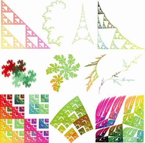
Figure 4.5 Attractors of IFSs belonging to similitude geometry, Mobius¨ geometry and projective geometry are shown on the left, in the middle and on the right respectively. The pictures are coloured by IFS colouring.

Figure 4.4 shows IFS colouring of the attractors of two different just-touching IFSs. In both cases the attractor is a square and the IFS colour code is defined in Table 4.7. The IFS for the right-hand image is given by Table 4.3 while that for the left-hand image consists of four transformations, each of which maps the square into one of its quadrants.

Notice how the right-hand picture looks as though it is a continuous transformation of the left-hand picture. This illustrates what we call a ‘fractal transformation’; see Section 4.15. In this case the implied mathematical transformation is a homeomorphism. But it is not differentiable and does not provide a metric equivalence between the two pictures.

Figure 4.5 illustrates various attractors, belonging to different geometries, coloured using IFS colouring (in contrast with colour-stealing, which we come to

in Section 4.10.) Points that lie in the set of overlapping points of the attractor will tend to be grainy and to change continually as the chaos game progresses.

E x e r c i s e 4.6.1 Use the IFS colouring algorithm to render your example in Exercise 4.5.2.

4.7 The collage theorem

How does one go about finding an IFS, in a two-dimensional setting, whose attractor is equal to, or ‘looks like’, a given compact target set T R2? Sometimes we can simply spot a set of contractive transformations f1, f2, . . . , fN taking R2 into itself, such that

If so then the unique solution T to Equation (4.7.1) is the attractor of the IFS

{R2; f1, f2, . . . , fN }.

If T has properties which belong to a certain geometry then it makes sense to seek the required IFS among transformations that belong to that geometry. For example, if T is a polygon in R2 then it is a good idea to restrict attention to projective IFSs.

But in computer-graphical modelling, image approximation and biological modelling applications, it is often not possible to find an IFS, with a restricted number of transformations belonging to a given geometry, such that Equation (4.7.1) holds. Nonetheless, we may seek an IFS that makes Equation (4.7.1) approximately true. That is, we may try to make T out of transformations of itself. The following theorem gives an upper bound to the distance between the attractor of the resulting IFS and T . The upper bound depends only on the distance from T to F(T ).

T h e o r e m 4.7.1 (The collage theorem [5]) (i) Let (X, d) be a complete metric space. Let T H(X) be given and let ≥ 0 be given. Suppose that a hyperbolic IFS F = {X; f1, f2, . . . , fN } of contractivity factor 0 ≤ l < 1 can be found such that

Figure 4.6 Illustrations of the collage theorem. The target set T is the leaf at top left. Next to it are shown three different collages of T , superimposed on T . Below each collage is shown the attractor of the corresponding projective IFS, also superimposed on T . Each attractor is rendered in four colours, showing how it may be seen as a union of transformations of itself.

f2, . . . , fN ; p1, p2, . . . , pN } with average contractivity 0 ≤ l < 1 can be found such that

dP (υ, F(υ)) ≤ ,

where dP denotes the Monge–Kantorovitch metric on P(X). Then

dP (υ, μ) ≤ ,

1 − l

where μ is the measure attractor of the IFS.

The collage theorem is an expression of the general principle that the attractor of a hyperbolic IFS depends continuously on its defining parameters, such as the coefficients in an IFS code. In practice, once we have an IFS whose attractor A resembles a given target T we can adjust the parameters in the IFS code to move A closer to T . Here you might find it useful to recall our discussion, in Section 1.12, of paths of steepest descent for the Hausdorff distance between two sets.

The process of seeking a small collection of ‘simple’ contractive transformations with which to form a collage of a given target set can be very surprising and rewarding. When preparing to write this section, I chose the leaf shown in Figure 3.1 to define the target set T . The digital picture was photographed several years ago beside Lake Padden in Washington State. So, restricting myself to four projective transformations, I made the illustrative collages shown in Figure 4.6. Then I realized that it was more efficient to use only three leaves, in a different type of configuration; see Figure 4.7.

Figure 4.7 From left to right this illustrates a target set, a collage and the corresponding attractor. In contrast with Figure 4.6, here only three transformations are used. You can probably find an even better approximation.

Next, I was further rewarded by finding a nearby IFS of three similitudes of great simplicity, namely

This IFS is also overlapping, and it is at first sight hard to see that its attractor, shown in Figure 4.8, is the union of three similitudes applied to itself. But it is. This attractor, while being quite close to T in the Hausdorff metric, possesses a completely different topology from T . I think that it is very beautiful because of the diversity of shapes that it contains. Does it suggest a model for the way in which the veins in the leaf grew?

The same idea of making collages applies equally well to the approximation of a given target set T using an orbital set or to the approximation of a given probability measure, or a picture of one, either by using the measure attractor of an IFS with probabilities or by using an orbital measure. Variants of the collage theorem have been applied to fractal image compression, fractal interpolation and vector IFS image modelling. See for example [9], [38], [97] and references therein.

We do not know of a good analogue to the collage theorem for orbital pictures or for fractal tops. This is the case despite the fact that, in practice, perhaps somewhat intuitively and perhaps only in the case of suitable target pictures, it seems possible to manipulate orbital pictures and rendered fractal tops so that they ‘look like’ the target.

Notice that approaches based on the collage theorem do not, per se, provide a control of fractal dimension or a topology of the approximate attractor. The topology and the fractal dimension of features of attractors may vary wildly with tiny changes in parameters, unless constraints are imposed. In fractal interpolation, the approximating IFS is constrained so that its attractor is the graph of a continuous