

Ohrimenko+ / Barnsley. Superfractals
.pdf200 |
Semigroups on sets, measures and pictures |
|||||
and |
|
(x) |
if x |
DP1 |
|
D , |
P1 P2(x) = P2 |
|
|||||
|
P1 |
(x) |
if x |
D |
, |
|
for all x DP1 P2 |
and for all P1, P2 . |
|
P2 |
\ P1 |
||
|
|
|
|
|||
We will use the tops union repeatedly in later sections, as well as here. We say that two segments or pictures are disjoint if their domains are disjoint. Given P1, P2 we define P1\P2 to be the picture whose domain is DP1 \DP2 and whose values are given by
(P1\P2)(x) = P1(x) for all x DP1\P2 .
E x e r c i s e 3.2.10 Verify that the binary operation is associative but not commutative.
E x e r c i s e 3.2.11 Let f : X →X be one-to-one. Prove that
f (P1 P2) = f (P1) f (P2) |
for all P1, P2 . |
|
E x e r c i s e 3.2.12 |
Let f : X →X be one-to-one. Prove that |
|
f (P1\P2) = f (P1)\ f (P2) |
for all P1, P2 . |
|
E x e r c i s e 3.2.13 |
Show that |
|
P1 P2 = P1 (P2\P1) |
for all P1, P2 . |
|
Notice that we can decompose a picture P into two segments P1 and P2 by choosing two domains DP1 and DP2 such that DP = DP1 DP2 . We have not required that the segments have disjoint domains. Now we define two pictures P1 : DP1 → C and P2 : DP2 → C by
Pk (x) = P(x) for all x DPk and for k = 1, 2. |
(3.2.2) |
It follows that these two pictures agree for all x DP1 ∩ DP2 , and consequently that
P = P1 P2 = P2 P1.
More generally, if two pictures P3 and P4 are such that they disagree at some point belonging to the intersection of their domains, then
P3 P4 = P4 P3.
D e f i n i t i o n 3.2.14 The semigroup (, ) is called the tops semigroup. Given , the smallest sub-semigroup of (, ) that contains is called the tops semigroup generated by .
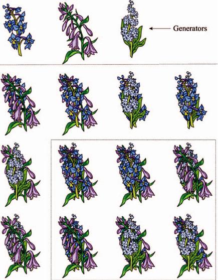
Figure 3.7 illustrates the pictures in the tops semigroup generated by three segments.
3.2 Semigroups |
201 |
Figure 3.7 Illustration of the tops semigroup generated by the three pictures in the upper row. The attractor A of this semigroup is represented by the six pictures at the lower right. Verify that if P and Q A then P Q A .
T h e o r e m 3.2.15 Let denote the tops semigroup generated by the finite set of pictures {P1, P2, . . . , PN } . Then is a finite set. Define fi : → by fi (P) = Pi P for all P and define F : S( ) → S( ) by
F(B) = f1(B) f2(B) · · · fN (B) for all B S( ),
202 |
Semigroups on sets, measures and pictures |
where the points of S( ), the space of subsets of , each consist of a set of pictures. Then there exists a unique point A S( ), i.e. a set of pictures, such that
|
|
|
|
|
|
|
|
|
|
|
|
|
|
|
|
A = F(A) |
|
|
|
|
|
|
|
|
||||
and moreover |
|
|
|
|
|
|
|
|
|
|
|
|
|
|
|
|
|
|
|
|
|
|
|
|||||
|
|
|
|
|
|
|
|
|
|
|
|
|
|
lim |
F◦k (B) |
= |
A |
|
|
|
|
|
|
|||||
|
|
|
|
|
|
|
|
|
|
|
|
|
|
k |
→∞ |
|
|
|
|
|
|
|
|
|
|
|
||
for all B S( ). |
|
|
|
|
|
|
|
|
|
|
|
|
|
|
|
|
|
|
|
|||||||||
|
|
|
|
|
|
|
|
|
|
|
|
|
|
|
|
|
◦ · · · ◦ fσ|σ | for all |
|||||||||||
|
P r o o f |
Let A = {1, 2, . . . , N } and define fσ = fσ1 |
◦ fσ2 |
|||||||||||||||||||||||||
|
= |
|
· · · |
|
| |
| |
|
|
A |
|
|
|
|
|
|
|
|
|
|
|
|
|
|
|
|
|
|
|
σ |
|
σ1σ2 |
|
|
σ σ |
|
|
. Then |
|
|
|
|
|
|
|
|
|
|
|
|
|
|
|
|||||
|
|
f |
σ |
(P) |
= |
P |
σ1 |
|
P |
σ2 |
· · · |
P |
σ|σ | |
|
P |
|
for all σ |
|
|
|
, P |
|
. |
|||||
|
|
|
|
|
|
|
|
|
|
|
A |
|
|
|||||||||||||||
It is readily verified that |
|
|
|
|
|
|
|
|
|
|
|
|
|
|
|
|
|
|||||||||||
|
|
|
|
|
|
|
|
|
|
|
|
f |
σ |
= |
f |
σ |
for all σ |
|
, |
|
|
|
|
|
|
|||
|
|
|
|
|
|
|
|
|
|
|
|
|
|
|
|
|
|
A |
|
|
|
|
|
|
||||
|
|
|
|
|
|
|
|
|
|
|
|
|
|
|
|
|
|
|
|
|
|
|
|
|
|
|
|
|
where σ is obtained from σ by deleting all but the leftmost occurrence of each symbol in A, so that for example
f132142 = f1324, f1222222 = f12 and f111121 = f12.
From Exercise 3.2.6 we know that every element of can be written in the form
Pσ1 Pσ2 · · · Pσ|σ | , |
(3.2.3) |
for some σ A. So it follows that every element of can be written as in Equation (3.2.3) with |σ | ≤ N , which tells us that is a finite set. It also follows that
σ |
|
, |
|
|
|
· · · fσ|σ | |
|
|
F◦(N +l)(B) = |
A |
| |
|= |
+ |
fσ1 |
fσ2 |
(B) |
|
|
|
|
|
|
||||
|
|
σ |
|
N l |
Pσ1 Pσ2 · · · PσN |
|||
= |
|
|
|
|||||
σ Perm(1,2,...,N )
for all l = 0, 1, 2, . . . , where Perm(1, 2, . . . , N ) denotes the set of strings σ , of length N , all of whose components are distinct.
D e f i n i t i o n 3.2.16 The set of pictures A defined in Theorem 3.2.15 is called the attractor of the tops semigroup generated by the finite set of picture segments {P1, P2, . . . , PN }.
The attractor A of the tops semigroup illustrated in Figure 3.7 is represented by the set of six pictures at the lower right.
Notice the following random iteration algorithm, which may be used to sample A. This description is informal. Let {F1, F2, F3} denote the three pictures

3.2 Semigroups |
203 |
in the top row of Figure 3.7, which generate the semigroup. Define a sequence of pictures P1, P2, P3, . . . by choosing P1 = Fσ1 and
Pn+1 = fσn (Pn ) = Fσn Pn for n = 1, 2, . . . , |
|
||||
where, for each n, |
independently of all other choices, σ |
n1= |
1 with probability 1 |
, |
|
|
1 |
6 |
|
||
σn = 2 with probability |
2 and σn = 3 with probability 3 . Look at the sequence |
||||
P1, P2, P3, . . . What will we see? The theory of Markov processes, see for example [37], Chapter XV, tells us it is almost certain, after some finite number of iterations N , that we will see Pn A for all n ≥ N . That is, the random sequence is ‘attracted’ to A. Moreover, with very high probability, the sequence of pictures will then behave ‘ergodically’, jumping around from picture to picture of the attractor, spending on average a certain fixed fraction of the ‘time’ on each element of the attractor. This highly probable eventual behaviour of the sequence of pictures is referred to as a stationary state of the Markov process.
More precisely, the possible pictures on the attractor are F1 F2 F3, F2 F1 F3, F3 F2 F1, F1 F3 F2, F3 F1 F2 and F2 F3 F1, which may be labelled 1, 2, 3, 4, 5 and 6, respectively. Then the probability of transition from picture i to picture j on the attractor is pi, j , where ( pi, j ) is the stochastic matrix
|
|
|
1 |
1 |
1 |
0 |
1 |
0 |
|
|
|
1 |
1 |
0 |
|||||
|
|
|
6 |
2 |
0 |
0 |
3 |
0 |
|
|
|
|
|
|
|
|
|||
|
|
6 |
2 |
1 |
1 |
|
1 |
||
|
|
|
|
|
3 |
|
|
|
|
P |
|
0 |
0 |
3 |
6 |
0 |
2 |
||
= |
|
0 |
1 |
0 |
1 |
1 |
0 |
. |
|
|
|
2 |
6 |
3 |
|
||||
|
|
|
|
|
|
|
|||
|
|
|
0 |
0 |
0 |
1 |
1 |
1 |
|
|
|
|
6 |
3 |
2 |
|
|||
|
|
|
|
|
|
|
|
|
|
|
|
|
1 |
0 |
1 |
0 |
0 |
1 |
|
|
|
|
6 |
|
3 |
|
|
2 |
|
The stationary state is described by the unique vector of probabilities
p = ( p1, p2, p3, p4, p5, p6)
such that
p P = P, pi > 0 for i = 1, 2, . . . , 6, |
6 |
|
|
|
|
pi = 1. |
(3.2.4) |
i=1
The number pi gives the average fraction of the pictures in the random sequence P1, P2, P3, . . . equal to the ith picture on the attractor; that is, almost always,
i = |
K |
K −1 |
{ |
1 |
2 |
3 |
, . . . , P |
K } |
. |
p |
lim |
|
number of times picture i occurs in P |
, P |
, P |
|
→∞
On solving Equation (3.2.4), using the Maple engine in [87], we find that
p = 101 , 16 , 14 , 151 , 121 , 13 .

204 Semigroups on sets, measures and pictures
We may think of this stationary state as being described by a probability measure
μ on the field generated by the pictures, with μ(F1 F2 F3) = 101 , μ(F2 F1
F3) = 16 , μ(F3 F2 F1 F1 F3 F2) = 14 + 151 and so on.
Thus we see how one may sample the elements of a semigroup by means of random iteration, actually a Markov process, thereby learning something about the semigroup. In fact, in this case, what we ‘see’ are elements of the attractor of the semigroup, sampled according to a certain probability distribution on the attractor.
E x e r c i s e 3.2.17 Choose the probabilities in the above discussion to be σn = 1 with probability 101 , σn = 2 with probability 15 and σn = 3 with probability 107 . Estimate the probability that P100 = F1 F2 F3.
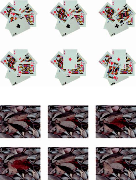
Another example of a tops semigroup is given in Figure 3.8. Here, the semigroup is generated by pictures of the playing cards A , Q , Q♠, K♥, J and A ♣, each positioned at a fixed angle. Again we may assign probabilities to the pictures and then sample the semigroup by means of the random iteration algorithm. This example provides a visual note of the connection between semigroups of pictures and probability theory.
Figure 3.9 shows members of the attractor of a tops semigroup generated by pictures of fallen leaves. Following the above discussion, we see how it is possible to generate probability measures on spaces of pictures, and how we may sample such spaces, even when they are vast, by means of random iteration.
E x e r c i s e 3.2.18 Let Pi for i = 1, 2, 3, 4. Verify that
|
P2 |
(x) |
if x |
D2 |
:= |
|||
|
P1 |
(x) |
if x |
|
D1 |
: |
|
|
(P1 P2 P3 P4)(x) |
|
|
if x |
= |
||||
|
P (x) |
|
D |
3 |
: |
= |
||
|
= 3 |
|
|
|
|
|||
|
P4(x) |
if x D4 := |
||||||
|
|
|
|
|
|
|
|
|
DP1 , DP2 \D1, DP3 \D2, DP4 \D3.
The following exercise gives an example of how to embed the semigroup (S(R2), ) in the tops semigroup ( C(R2), ) in such a way that the operation of on S(R2) is equivalent to the operation of on the embedded elements inC(R2).
E x e r c i s e 3.2.19 Let the colour space C be such that 0 C and 1 C. Let
P0 : R2 → C denote an endless ‘blank’ picture, that is, P0(x) = 0 for all x R2. Let S1, S2 S(R2) and let PSi : Si → C be defined by PSi (x) = 1 for all x Si . Let χS denote the characteristic function of S R2. Show that
(i)PSi P0 = χSi for i = 1, 2;
(ii)PS1 PS2 = PS2 PS1 = PS1 S2 ;
(iii)if ξ : S(R2) → C(R2) is defined by ξ (S) = PS for all S S(R2) then ξ is one-to-one and hence an embedding, and moreover
ξ (S1 S2) = PS1 PS2 for all S1, S2 S(R2).
3.2 Semigroups |
205 |
Figure 3.8 Pictures belonging to the attractor of the tops semigroup generated by pictures of A , Q , Q♠, K♥, J and A♣.
Figure 3.9 Pictures of the ‘forest floor’ belonging to a tops semigroup generated by pictures of individual leaves.
The surfaces of some moons are pockmarked with disk-shaped craters. Model pictures of these surfaces may be generated by pretending that meteors of randomly different sizes hit the moon at randomly different places, overlaying craters on craters. Such pictures may be treated as random fractal pictures generated
206 |
Semigroups on sets, measures and pictures |
by tremas, a word apparently coined by Mandelbrot; see [64], pp. 305–8. Vast collections of such pictures may be explored by random iteration.
E x e r c i s e 3.2.20 See if you can find, on the internet, simulations of pictures of falling dead leaves; use a search engine such as Google. What is the difference between the behaviour, over time, of pictures of fallen leaves on a glass table, on which they steadily accumulate starting from a clean surface, viewed (a) from above and (b) from below?
Semigroups of measures
The sum of two Borel measures is a Borel measure. The weighted average of two probability measures on R2 is a probability measure on . Thus (P( ), ♥) is a semigroup of probability measures, where we define μ ♥ ν = 13 μ + 23 ν. If we think of μ and ν as greyscale pictures, then μ ♥ ν is a weighted average of the two pictures. Clearly μ ♥ ν =ν ♥ μ in general.
E x e r c i s e 3.2.21 Let S denote the sub-semigroup of (P( ), ♥) generated by two distinct measures μ0, μ1 P( ). Describe S. For example, think of μ0 and μ1 as greyscale pictures and then describe the set of pictures in S. Can you set up an
addressing function |
f : { |
0,1} → S? Better still, can you describe an addressing |
||||||||
function f : |
|
|
|
|
|
, where |
|
denotes the closure of |
|
? |
0,1 |
} |
→ S |
S |
S |
||||||
{ |
|
{0,1} |
|
|
|
|||||
3.3 Semigroups of transformations
Semigroups of transformations are central to this book because we use them to define and manipulate sets, pictures and measures. They play a key role in fractal geometry.
D e f i n i t i o n 3.3.1 A semigroup of transformations on a space X is a semigroup (S(X), ◦), where S(X) consists of transformations from X into X and where the binary operation is composition. That is, f ◦ g is the transformation defined by
f ◦ g(x) = f (g(x)) for all x X.
The composition of functions is an associative operation because
f1 ◦ ( f2 ◦ f3)(x) = f1( f2( f3(x))) = ( f1 ◦ f2)( f3(x)) = ( f1 ◦ f2) ◦ f3(x)
whenever f1, f2, f3 : X → X. We will tend to drop the explicit reference to the binary operation for semigroups when the operation is obvious, for example, the composition of functions. So we may say ‘S is a semigroup’ or ‘S(X) is a semigroup of transformations (on the space X )’. We will look mainly at semigroups of transformations on spaces, such as R2, that are related to pictures.
3.3 Semigroups of transformations |
207 |
Examples of semigroups of transformations
Here we introduce the main semigroups of transformations that we need for fractal geometry and superfractals. The most important of these for the purposes of this book are IFS semigroups, in particular those built from projective and Mobius¨ transformations. Elsewhere we use these semigroups to form semigroup tilings, fractal sets and measures, fractal tops and superfractals.
Semigroups of linear transformations
The set of linear transformations that map a linear space such as R2 into itself forms a semigroup, because if both f and g are linear transformations then so is f ◦ g. If two linear transformations f1 and f2 are represented by matrices A1 and A2 respectively then it is readily verified that the linear transformation f1 ◦ f2 is represented by the matrix A1 · A2. So we may use the semigroups of matrices to study semigroups of linear transformations, and vice versa.
Recall that the domain of a transformation is an important part of its definition. So, for example, let T denote the set of linear transformations that map a certain set D R2 into itself. Then S := { f |D : f T } is a semigroup. Notice too that there is no requirement of invertibility on the transformations in a semigroup. Let f T . Then the transformation f |D : D → D may not be one-to-one for one of the following reasons: (i) there are points outside D that are mapped by f into D; (ii) the determinant of the matrix that represents f may be zero.
Semigroups of M¨obius transformations
The composition of two Mobius¨ transformations acting on the space R2 {∞}, or equivalently C, is a new Mobius¨ transformation. So the set of Mobius¨ transformations on R2 {∞} is an example of a semigroup. Interesting sub-semigroups of Mobius¨ transformations are generated by small sets of Mobius¨ transformations with integer coefficients.
Suppose that M is a set of Mobius¨ transformations that map a domain D R2 {∞} into itself. Then the set of transformations obtained by restricting the transformations of M to D is a semigroup. Although a Mobius¨ transformation is always invertible, the corresponding transformation restricted to D may not be one-to-one.
Semigroups of projective transformations
The set of projective transformations acting on R2 L∞ or RP2 forms a semigroup of transformations. Sets of projective transformations with a common restriction, for example those that share a fixed point or map a particular subset such as a conic section into itself, also form semigroups. Semigroups of projective transformations, restricted to a domain that they map into itself, can also be constructed.
208 |
Semigroups on sets, measures and pictures |
Again, although a projective transformation is always invertible, such restricted transformations may not be.
Semigroups of transformations on code spaces
It is possible to form diverse semigroups of transformations on a code space. We note in particular the semigroup of transformations generated by the shift transformation, which is not invertible when |A| > 1.
E x e r c i s e 3.3.2 For each σ A the corresponding branch transformation fσ : A → A is given by fσ (ω) = σ ω = σ1σ2 · · · σ|σ |ω1ω2 · · · for all ω A. Show that { fσ : σ A} is a semigroup of transformations.
IFS semigroups
An iterated function system, or IFS, consists of a finite sequence of transformations that map from a space to itself. An IFS may be denoted by
{X; f1, f2, . . . , fN },
where fi : X → X for i = 1, 2, . . . , N and N ≥ 1 is an integer. Thus we may refer to ‘the IFS {X; f1, f2, . . . , fN }’. Please look back at Chapter 2, around Theorem 2.4.15, where we first introduced IFSs. Typically we consider IFSs in which the space X is a metric space, the transformations are Lipschitz or strictly contractive, i.e. L < 1, and there is more than one transformation. When the transformations are contractions and the space X is complete the IFS is called a contractive IFS. A contractive IFS is referred to as a ‘hyperbolic’ IFS in [9] and possesses a unique attractor, or fractal set, the fixed point of the associated contraction mapping on H(X). We will often denote the attractor set of a contractive IFS by the symbol A.
D e f i n i t i o n 3.3.3 An IFS semigroup is a semigroup of transformations generated by an IFS.
We will use the notation S{X; f1, f2,..., fN }, or S{ f1, f2,..., fN }(X) or more briefly S{ f1, f2,..., fN }, to denote the IFS semigroup generated by the IFS {X; f1, f2, . . . , fN }. In this chapter we are interested in the orbits of sets, measures and pictures under
IFS semigroups and in the sets, measures and pictures that can be constructed from these orbits.
E x e r c i s e 3.3.4 Let (X, d) be a metric space. Show that the set of Lipschitz transformations on X forms a semigroup.
E x e r c i s e 3.3.5 Let (X, d) be a metric space. Show that the set of Lipschitz transformations on X with Lipschitz constant L < 1 forms a semigroup.
E x e r c i s e 3.3.6 Let (X, d) be a metric space. Construct an example to show that the set of Lipschitz functions with a fixed Lipschitz constant L > 1 does not in general form a semigroup.
3.3 Semigroups of transformations |
209 |
From this point, if this is new material for you, you might like to omit the final three examples of semigroups and skip ahead to the next subsection.
Semigroups of rational transformations on the Riemann sphere
There are many types of semigroups of tranformations that act on ‘flat’ spaces such as R2. We note in particular that the set of rational functions of a complex variable, that is, ratios of complex polynomials in z C, forms a semigroup of transformations on the Riemann sphere. Such semigroups are related to complex analytic dynamical systems and to graceful families of fractals such as Julia sets. The set of complex polynomials and the set of rational functions of degree 1, namely the Mobius¨ transformations, are each sub-semigroups. Again, new semigroups may be obtained by restricting the domains of the transformations.
Semigroups associated with dynamical systems
There is a close relationship between dynamical systems and fractals, and techniques used in dynamical systems theory are useful in connection with IFSs and IFS semigroups. Conversely, fractal geometry informs dynamical systems theory.
The study of the semigroup generated by a single transformation f : X → X is essentially the study of the corresponding dynamical system, denoted by {X; f }. Studies of dynamical systems tend to focus on the case where f is invertible – see for example [56]. The orbit of a point x0 X under the dynamical system {X; f } is the sequence of points {xn = f ◦n (x0) : n = 0, 1, 2, . . . }; note that the orbit includes the initial point x0. Studies of dynamical systems are primarily concerned with the structure of their orbits, the limiting behaviour of their orbits, ergodic properties, recurrence properties (dealing with questions such as ‘When does an orbit return arbitrarily close to its starting point?’) and properties which are invariant under changes of coordinates.
Topological dynamics, for example, is concerned with groups of homeomorphisms and semigroups of continuous transformations on compact metric spaces. Dynamical systems theory uses in particular the study of dynamical systems on code space A, called symbolic dynamical systems, together with mappings between code space and other spaces, for example R2, to explain aspects of the behaviour of dynamical systems acting on the latter spaces.
Semigroups associated with autonomous systems
One notable circumstance where semigroups of transformations arise is in connection with any model physical system whose state x(t) at time t ≥ 0 can be determined fully from a knowledge of both its state at any earlier time s ≥ 0 and the time elapsed, t − s. We call such systems autonomous.
An autonomous system always behaves in the same way when it is started off in the same way; it runs to its own clock, not an external one. Indeed a perfect