Ohrimenko+ / Barnsley. Superfractals

wind-up clock is an example of an autonomous system. Autonomous systems occur frequently in the physical sciences; any experiment in physics which can be repeated over and over again to produce the same behaviour, regardless of the date and time, and which may be initialized at any of its states may be represented by such a model. Often the model involves an array of integro-differential equations that incorporate the model assumptions, physical laws, etc. which govern its behaviour. Some of these systems model physical processes that influence the shape and look of the world around us.

Autonomous systems may be associated with conservation laws and invariance properties in fluid dynamics, classical mechanics, electrostatics and so on. We are interested in them because the colour and intensity of the light emitted or reflected by real-world objects moving in an approximately autonomous system, such as waves on the sea or clouds in the sky or the rings of Saturn, finds its way into real-world pictures; we expect to find some sort of trace or record of these systems in invariance properties of parts of pictures under appropriate semigroups of transformations.

Let X denote the set of possible states of an autonomous system. It could describe, for example, the height of a plant, the coordinates and momentum of a particle, the number of sharks and fishermen in a model for interacting species, the positions of the hands on a clockface or possible combinations of colours and forms in a picture that changes with time according to certain rules.

We define Ft : X → X to be the transformation that maps the state of an automous system at time t = 0 to its state at time t ≥ 0. The transformation Ft is sometimes called an evolution operator. Since Ft (Fs (x)) = Ft+s (x) for all x X, it follows that

is a semigroup of transformations. Since this semigroup depends upon a single parameter, t, it is called a one-parameter semigroup.

Let Ft : X → X with t ≥ 0 be an evolution operator, let x X and let O(x) be the orbit of x; see Definition 3.3.8 below. When X R2 the set of orbits of an autonomous system may provide what is called a phase portrait of the system. We think of a phase portrait as being a picture, maybe in black and white, showing the orbits of many different points simultaneously. We notice that

So an autonomous system yields a semigroup of transformations, Equation (3.3.1), and a collection of sets, Equation (3.3.2), each of which is mapped into itself by every transformation of the semigroup. We can think of some phase portraits as being pictures that are invariant under semigroups of transformations.

E x e r c i s e 3.3.7 Let X = R2 and (x, y) = (x(t), y(t)) R2 evolve according to the pair of differential equations

subject to the initial condition (x(0), y(0)) = (x0, y0), where α, β > 0 and (x0, y0) is any point in R2. Show that the corresponding evolution operator Ft : R2 → R2 is defined by the 2 × 2 matrix

Verify that Ft · Fs = Ft+s . Show that, for all points (x, y) on any orbit of the system,

Describe subsets of R2 that are mapped into themselves by all transformations of the semigroup.

Orbits of semigroups

D e f i n i t i o n 3.3.8 An orbit of a semigroup S(X) is a subset of X of the form

O(x) = {x} { f (x) : f S(X)}

for some x X. O(x) is called the orbit of the point x. A semigroup is said to be discrete iff the orbit O(x) X consists of isolated points for all x X. A semigroup is said to be continuous iff, for any given x X, there is a continuous function f : [0, ∞) → X such that the orbit O(x) can be written in the form O(x) = { f (t) : t [0, ∞)}.

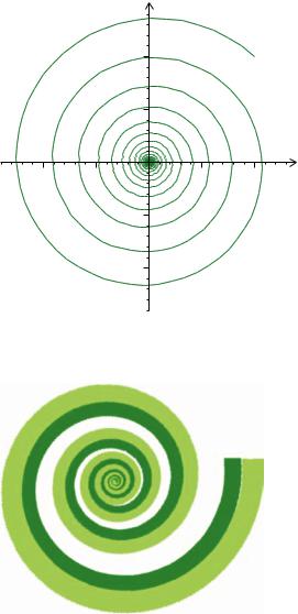
An example of an orbit O(x) of a point x under a continuous semigroup is illustrated in Figure 3.10. The semigroup of transformations is { fθ : θ [0, ∞)}, where fθ : R2 → R2 is defined by

Figure 3.10 Orbit of the point (1, 1) under the continuous semigroup of transformations defined in Equation (3.3.6).

Figure 3.11 Example of a picture that is invariant under a continuous semigroup of transformations.

In the figure, r = 0.975 and x = (1, 1). In this case the orbit is actually invariant under the semigroup, that is,

O(x) = { fθ (O(x)) : θ [0, ∞)}.

See also Figure 3.11.

A visual example of an orbit of a semigroup is the set of points defined by the tips of the green leaves in Figure 3.3. Clearly in this case we are dealing with a discrete semigroup. See also Figure 3.12.

Show that { fα : α R} is a continuous semigroup and that { fα : α Z} is a discrete semigroup.

Sketch the orbit of the point (1, 1) under the semigroup of transformations { fθ :

θ [0, ∞)}.

Consider the IFS semigroup S{ f }(X) generated by a single transformation f : X → X. We define f ◦0(x) = x for all x X, f ◦1 = f and f ◦(n+1) = f ◦ f ◦n

for n = 1, 2, 3, . . . Then

S{ f }(X) := { f ◦n : n = 0, 1, 2, . . . }.

Clearly

f ◦n ◦ f ◦m = f ◦(n+m) for all m, n = 0, 1, 2, . . .

In this case the orbit O(x) of the point x X under the semigroup S{ f }(X) is

O(x) = { f ◦n (x) : n = 0, 1, 2, . . . }.

Notice that, knowing the IFS, we can treat this orbit as a sequence.

Suppose that the semigroup S{M}(R2) is generated by a linear transformation M : R2→ R2 represented by the matrix M. Then, since

( f ◦n (x, y))T = Mn x , y

it follows that

S{M}(R2) = {Mn : n = 0, 1, 2, . . . }

where M0 := I , the identity matrix.

E x e r c i s e 3.3.11 Plot the orbit of the point (1, 1) R2 under the semigroup of transformations S{M}(R2), where M is the linear transformation represented by

Figure 3.12 What is the orbit of the top left corner of the second largest frame in this picture, under the semigroup of transformations implied by this picture?

Notice that O(C) is a set of sets of points. We will write

P = O(C)

to denote the union of all the sets in the orbit O(C). We call P = O(C) the orbital set associated with the semigroup S(X) acting on the set C.

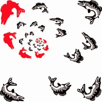
Orbits of sets under semigroups of transformations are illustrated in Figures 3.13–3.16 and 3.18. Notice that the sets in the orbits may have nonempty intersections or they may all be separated from one another. Notice too that there is no requirement that the set C be connected; for example, C could be the union of the fish in the four corners of Figure 3.13.

When X is a ‘flat’ space such as R2 we think of P as a black-and-white picture. The following theorem says that this picture is the union of transformed copies of itself together with the set C. In order to describe this picture, we need to know only C and the set of transformations that generate the IFS. In this context we sometimes call C a condensation set; see for example [9] or [46]. We will also, later, refer to condensation pictures and condensation measures. Be careful not to confuse ‘condensation set’ with ‘the set of condensation points of a set’. The latter refers, in other texts, to an unrelated concept.

T h e o r e m 3.4.2 Let O(C) denote the orbit of a nonempty subset C of X under the IFS semigroup S{ f1, f2,..., fN }(X). Let P = O(C). Then P obeys the

Figure 3.14 Two different semigroup tilings of orbital sets generated by a single projective transformation f acting on a condensation set C , the leafy spring at the centre of the figure. The intersection of any filled rectangle that does not meet C with the orbital picture is the image, under this transformation, of the intersection of a filled quadrilateral with the orbital picture.

Theorem 3.4.2 says that the orbital set P is a fixed point of the transformation FC : S(X) → S(X) defined by

FC (B) = C f1(B) f2(B) · · · fN (B)

for all B S(X), and that

O(C) = O(P).

When the underlying space X is a compact metric space, C is compact and the IFS consists of strictly contractive transformations, we have FC (H(X)) H(X), where H(X) is the space of nonempty compact subsets of X. In this case, if we restrict FC to H(X) then it becomes a strict contraction with respect to the Hausdorff metric. In this case, as in Theorem 2.4.15, the orbital set P is unique in H(X). Moreover, this unique fixed point depends continuously on the transformations in the IFS and on the condensation set C. In other words, in this strictly contractive case, if