Ohrimenko+ / Barnsley. Superfractals

Figure 2.45 This illustrates the locations of the three fixed points (0, 0), (0, 1) and (1, 0) of the canonical family of projective transformations Pa,b that take (1, 1) to (a, b). This family of transformations leaves fixed the straight line passing through (0, 0) and (0, 1). It also leaves fixed the straight lines through (0, 0) and (1, 0) and through (1, 0) and (0, 1).

from what an affine transformation does, can be understood by considering how Pa,b acts on pictures.

E x e r c i s e 2.7.6 In the above discussion, let D be a fourth point in the domain of P such that no three of A, B, C, D are collinear, and let D be a point in the domain of P such that no three of A , B , C , D are collinear. Show that (a, b) can be choosen in such a way that P(D) = D . Thus devise a ‘move-four-points’ algorithm for adjusting projective transformations, analogous to the ‘move-three- points’ algorithm described in Figure 2.30.

It is readily verified that

Pa,b(0, 0) = (0, 0), Pa,b(1, 0) = (1, 0) and Pa,b(0, 1) = (0, 1).

Moreover each transformation in the family maps each of the lines given by x = 0, y = 0 and x + y = 1 onto itself; it maps the line L D given by

(a − 1)x + (b − 1)y + 1 = 0

to the line at infinity and L∞ to the line L R given by

Figure 2.46 The dance of the conics! A projective transformation always maps conic sections into conic sections. Each of the two panels illustrates the family of conic sections (x + y − 1)2 + γ x y = 0 where γ R. Each projective transformation Pa,b in Equation (2.7.3) maps this family into itself.

Each member of this family of projective transformations has the remarkable

one-to-one onto itself. We now sketch the proof of this fact. Let (x0, y0) R2 and suppose that (x0, y0) Cγ . Let Pa,b(x0, y0) = (x, y). Then

=(1/a − 1)x + (1/b − 1)y + 1 , (1/a − 1)x + (1/b − 1)y + 1

and substituting into (x0 + y0 − 1)2 + γ x0 y0 = 0, to formally eliminate x0 and y0, we obtain

(x + y − 1)2 + γ x y = 0, ab

from which it follows that

Pa,b(Cγ ) = Cγ /(ab).

This completes the demonstration.

Figure 2.46 illustrates the family of conic sections given by Equation (2.7.4), and shows how some of them are mapped into others by members of the family of projective transformations Pa,b.

Figure 2.47 The top left panel shows a picture P, in various colours, of parts of some of the conic sections Cγ , defined by Equation (2.7.4), lying within the window −3 ≤ x ≤ 3, −3 ≤ y ≤ 3. The other three panels show, superimposed upon the original set of contours, the picture Pa,b (P) superimposed upon P for (a, b) = (1.1, 1.1) (top right), (a, b) = (0.9, 1.1) (bottom right) and (a, b) = (1.1, 1.1) (bottom left). You can see quite clearly that Pa,b maps the underlying striated pattern onto itself, albeit, in these cases, that the colours are not preserved. The straight lines were added afterwards to show to where part of the boundary of the original picture is mapped.

In particular, if ab = 1 then Pa,b maps each conic section Cγ onto itself. So in this case, for example, the top left panel of Figure 2.47 represents an invariant picture for Pa,b because not only is the striated pattern preserved but the colours of the contours, before and after, are preserved too. Another example of a picture that is invariant under Pa,b when ab = 1 is shown in Figure 2.48.

E x e r c i s e 2.7.7 Show that, when γ = 1, Cγ is the circle of radius 1 centred at

(1, 1) R2.

Figure 2.48 Part of a picture that is, to an approximation, invariant under a family of projective transformations.

When ab = 1 and 1 > a > 0, the projective transformation Pa,b maps the disk D of radius 1 centred at (1, 1) onto itself. Points are attracted towards the fixed points (1, 0) and repelled by the fixed point (0, 1). Any picture P with domain D is transformed to a new picture with domain D. What is the relationship between P and Pa,b(P)? We can think of Pa,b as sweeping lines of points around in a circle centred at (0, 0) in such a way that the points on the lines follow elliptical paths, each concentric ellipse passing through the two fixed points (1, 0) and (0, 1). Straight lines are preserved, but so are these ellipses. This effect is illustrated in Figure 2.49, where we have chosen a = 0.5 and b = 2.0.

E x e r c i s e 2.7.8 Compare the disk-preserving transformation illustrated in Figure 2.49 with that illustrated in Figure 2.35. What properties do the two transformations have in common?

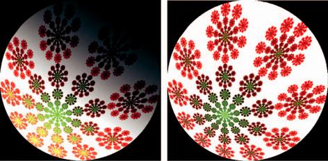
Figure 2.49 The projective transformation applied here maps a disk onto itself. Flowers in the picture are swept along elliptical paths away from one fixed point and towards the other. Where are the fixed points?

The way in which Pa,b maps the family of conic sections {Cγ : γ R} onto itself illustrates general properties of projective transformations in relation to conic sections.

D e f i n i t i o n 2.7.9 A non-degenerate conic section is a set of points C R2 L∞ given by an equation of the form

Ax2 + Bx y + C y2 + F x + Gy + H = 0, where A, B, C, F, G, H R

(2.7.5)

with A =0, or B =0 or C =0, such that C does not contain a straight line or a single point. If Equation (2.7.5) describes an ellipse or circle then C includes no points on L∞. If Equation (2.7.5) describes a hyperbola then C includes the two points on L∞ at which the asymptotes of the hyperbola intersect L∞. If Equation (2.7.5) describes a parabola then C includes the point at which the axis of the parabola intersects L∞.

It is readily verified that if C is a non-degenerate conic section and P : R2 L∞ → R2 L∞ is a projective transformation then P(C) is also a non-degenerate conic section.

The following theorem tells us not only that we can find a projective transformation that maps any given non-degenerate conic section onto any other one but also that we can do so in such a way that any three distinct points on the first conic can be mapped onto any three distinct points on the other conic, in any order.

T h e o r e m 2.7.10 Let C, C R2 L∞ be non-degenerate conic sections. Let three distinct points A, B, C C and three distinct points A , B , C C be

given. Then there exists a projective transformation P : R2 L∞ → R2 L∞ such that P(C) = C and P(A) = A , P(B) = B , P(C) = C .

P r o o f This follows from [25], p. 180, using the conventions adopted here regarding points on L∞.

E x e r c i s e 2.7.11 (i) Show that if P : R2 L∞ → R2 L∞ is a projective transformation with a fixed point Q R2 and a fixed line l R2 L∞ through Q, for which Q l, P(Q) = Q and P(l) = l, and if C is a non-degenerate conic section which is tangent to l at Q, then P(C) is a non-degenerate conic section which is tangent to l at Q. (ii) Use this result to deduce the formula in Equation (2.7.4) for a family of conic sections {Cγ : γ R}, which is invariant under the family of projective transformations {Pa,b : a, b R, ab =0} in Equation (2.7.3). Is this family {Cγ : γ R} unique? Or can you find another nontrivial family of conic sections which contains conic sections different from those in the family {Cγ : γ R} and which is invariant under Pa,b for all a, b R with ab =0?

In order to complete our understanding of how our special canonical family of projective transformations {Pa,b : a, b R, ab =0} acts on pictures, we mention

The eigenvectors of Pa,b(0, 0) are directed along the coordinate axes, with eigenvalues a and b. So when, for example, ab = 1 with 0 < a < 1 the fixed point (0, 0) is hyperbolic: any point on the x-axis sufficiently close but not equal to (0, 0) is transformed by Pa,b to a point even closer to (0, 0), while any point on the y-axis sufficiently close but not equal to (0, 0) is transformed by Pa,b to a point further away from (0, 0). Thus, a hyperbolic fixed point is attractive in some directions

Figure 2.50 A vector field associated with the family of projective transformations Pa,b . The crossed arrows represent the first-order linear approximations to Pa,b at the three fixed points, showing the eigenvalues and eigendirections. The grey arrows correspond to the case ab = 1 with 0 < a < 1, and indicate the directions in which points are moved along the conic sections when Pa,b is applied.

and repulsive in others; upon iterative application of the transformation in the vicinity of a hyperbolic fixed point, many points follow orbits that may initially be drawn towards the fixed point but eventually are repelled by it.

The eigenvectors of Pa,b(1, 0) are (1, 0)T and (1, −1)T , with eigenvalues a−1 and ba−1 respectively. So for ab = 1 with 0 < a < 1 the fixed point (1, 0) is repulsive: any point sufficiently close but not equal to (1, 0) is transformed by Pa,b to a point further away from (1, 0).

The eigenvectors of Pa,b(0, 1) are (0, 1)T and (1, −1)T with eigenvalues b−1 and ab−1 respectively. So for ab = 1 with 0 < a < 1 the fixed point (0, 1) is attractive: any point sufficiently close but not equal to (0, 1) is transformed by Pa,b to a point nearer to (0, 1). The situation is illustrated in Figure 2.50.

The linear operators in Equation (2.7.6) are useful in understanding how Pa,b transforms pictures. For example, suppose that P is an invariant picture for Pa,b. Then in the vicinity of a fixed point P must look approximately like an invariant

picture for the corresponding linear operator; that is, if we were to magnify P in the vicinity of (0, 0) we should see, within a finite fixed viewing window, what looks like part of an invariant picture for Pa,b(0, 0).

E x e r c i s e 2.7.12 What do the ‘local’ invariant pictures of the three linear transformations Pa,b(0, 0), Pa,b(1, 0) and Pa,b(0, 1) corresponding to the invariant picture in Figure 2.48 look like?

Projective transformations of measures

Let μ P(R2 L∞) be a measure that is absolutely continuous in the vicinity of a point X R2, with ‘density’ ρ in the vicinity of X . Let P : R2 L∞ → R2 L∞ be a projective transformation such that P(X ) R2. Then P(μ) is absolutely continuous in the vicinity of P(X ), with density

This remarkably simple formula, which is fun to verify, tells us that the factor by which brightness is scaled under projective transformation is constant on lines parallel to the line L D mapped by P to the line at infinity. This effect is easy to see in Figures 2.15 and 2.16, which show pictures of projective transformations applied to measures. The lines of constant scaling factor are clearly seen.

Figure 2.16 shows another effect also. When the intensity value of a colour component at a pixel is scaled so that the result would be greater than 255, the result is set to the value 255; we say that the brightness becomes saturated. This saturation effect can cause colours of pixels to become distorted as they become brighter, because upon scaling one of the colour components may reach the value 255 before the others.

Figure 2.51 shows a picture that is invariant under a projective transformation P : R2 L∞ → R2 L∞ of the form

P = Pa,bRPa−,1b,

where a = 1.5, ab = 1 and R is a rotation through π/5. Figure 2.51 also shows a closely related picture of a vector of measures, each of which is invariant under

P.

E x e r c i s e 2.7.13 Compare Figure 2.51 with Figure 2.17. How can you tell that Figure 2.51 does not represent a Mobius¨ transformation?

E x e r c i s e 2.7.14 Simplify Equation (2.7.8) in the case where P|R2 is an affine transformation. Show that Equation (2.7.7) is consistent with Equation (2.5.4) when P|R2 is a linear transformation.

Projective transformations on RP2

The most natural way to think mathematically and computationally about projective transformations is to represent them as acting on RP2. This greatly simplifies some aspects of understanding these transformations, though on its own it does not, in my experience, add much intuition to the specifics of how they act on pictures on R2 L∞. This may be because the detailed way in which a picture is deformed, when it is mapped from a sphere to a plane, can be hard to imagine.

D e f i n i t i o n 2.7.15 The projective plane is denoted by RP2. It consists of the set of straight lines in R3 that pass through the origin of coordinates, O = (0, 0, 0).

The points of RP2 are mathematical objects: each object consists of a set of points, namely a line, belonging to the underlying space R3.

E x e r c i s e 2.7.16 Show that x RP2 iff there exists a point l = (l1, l2, l3) R3, with l =O, such that

x = {(x1, x2, x3) R3 : (x1, x2, x3) = c · (l1, l2, l3) for some c R}.

Any point l = (l1, l2, l3) R3 with l =O defines uniquely a corresponding point in RP2, namely the line through O and l. We denote this line by the same

notation, l = (l1, l2, l3) RP2. The only difference is the space to which it is asserted that the point belongs.

D e f i n i t i o n 2.7.17 A projective transformation P : RP2 → RP2 is an invertible linear transformation P : R3 → R3 treated as acting on the set of straight lines in R3 through O.

Thus P : RP2 → RP2 is a projective transformation iff there exists an invertible linear transformation P : R3 → R3 such that

define the same projective transformation P : RP2 → RP2.

E x e r c i s e 2.7.20 Show that any projective transformation P : RP2 → RP2 maps RP2 one-to-one onto itself.

The space RP2 may be imagined to look something like a pin cushion full of pins, except that the cushion itself consists of a single point, the origin, and the pins are infinitely long and infinitesimally thin; we imagine that each pin has been stuck through the cushion and out the other side, protruding to infinity in both directions. Each pin represents a single point in the projective plane. Following Theorem 2.5.4, a projective transformation produces a rescaling in three orthogonal directions of the space containing the pins, possibly followed by a reflection and/or a rotation. Some bundles of pins are squeezed more tightly while others are expanded, as illustrated in Figure 2.52.

We now describe the relationship between projective transformations acting on RP2 and projective transformations acting on R2 L∞. Each point in RP2 is identified with a point in R2 L∞ in a one-to-one onto manner. Each line in R3 through O that intersects the plane

1 := {(x, y, z) : z = 1}

is identified by its point of intersection with 1. This represents ‘most’ of RP2 as a copy of R2. But some lines in R3 through O do not intersect 1, namely all the lines through O that lie in the plane

0 := {(x, y, z) : z = 0}.