Ohrimenko+ / Barnsley. Superfractals

some transformations in the above IFSs with an improper rotation such as (−x, y); see [23], vol. 1, p. 19.

In Figures 3.70, 3.72, and 3.73 we showed pairs of orbital pictures corresponding to three different crystallographic groups. In each case, basically the same condensation picture, P0, illustrated in Figure 3.70, is used. The units of the viewing windows on the right are larger, with the consequence that the condensation sets on the right are in effect larger than on the left. On the left the transformed copies of the condensation picture are non-overlapping and the result is a classical wallpaper pattern. On the right, however, some transformed copies of P0 overlap and the resulting pattern, almost a wallpaper pattern, varies subtly across the picture. By inspection, one finds that the pictures on the right are panellings of diversity greater than 4.

In Figure 3.74 the condensation picture represents our friend the buttercup. We have not shown here systematically the many types of wonderful orbital pictures that may be generated by the tiling groups. Great diversity, a wealth of different types of harmonious pictures, may be produced, for example merely by changing the ordering of the maps and the position and scaling of the condensation picture. Are modern wallpaper printing machinery and paper-hangers up to the task of decorating your dining room with orbital pictures?

Since any rigid transformation is an invertible affine transformation, euclidean geometry also displays all the properties of affine geometry, including fractal dimension.

Affine geometry

Two-dimensional affine geometry is defined by the group Gaffine, which consists of all invertible affine transformations acting on the space R2. Angles and distances are not preserved but triangles are mapped onto triangles, ellipses onto ellipses, hyperbolas onto hyperbolas, parabolas onto parabolas and parallel lines to parallel lines. The properties of being triangular, elliptical or parabolic etc. all belong to affine geometry. Since the transformations are also homeomorphisms, topological properties such as openness, compactness, connectedness, perfection etc. belong to affine geometry too. Moreover, since an invertible affine transformation is a metric transformation, fractal dimension is a property of affine geometry; see Section 1.14.

Let us say whimsically that a picture has the ‘modernist property’ iff it contains a domain whose boundary is a parallelogram, an elliptical feature, an open set coloured a certain shade of red (R = 242, G = 160, B = 148) and a subset, in brightest blue, whose boundary has fractal dimension 1.79. Then the ‘modernist property’ belongs to affine geometry.

IFS objects associated with affine IFSs inherit properties from affine geometry. For example, an affine orbital picture P may contain a global segment, made of

multiple panels and possessing distinctive features of parallel lines, cross-ratios and triangular structures, that is mapped by a transformation of the IFS onto a different segment of P with the same distinctive features. Such patterns may be repeated many times. Also, if the domain of the condensation picture is triangular then the boundaries of tiles and panels will be piecewise linear; and if the domain of the condensation set is constructed from finitely many pieces of hyperbolas then the domains of all the panels will be constructed from finitely many pieces of hyperbolas.

Also, affine IFS objects provide properties of affine geometry. In the same whimsical vein as above, let us say that a measure has the ‘affine orbital measure property’ iff it is an orbital measure generated by an IFS semigroup of affine transformations. Then the ‘affine orbital measure property’ belongs to affine geometry. You get the idea?

Some properties of affine geometry follow from the fact that it is a subset of projective geometry.

E x e r c i s e 3.7.12 Show that a geometry is defined by the set of affine transformations whose linear parts have determinants equal to +1. Show that area is a property of this geometry.

E x e r c i s e 3.7.13 Show that the set of similitudes, that is, affine transformations that preserve angles, yields a geometry. This geometry is called similitude geometry.

E x e r c i s e 3.7.14 Let A denote the set of affine transformations, on R2, of the special form

Let G denote an IFS group whose transformations all belong to A . Clearly, because G Gaffine the geometry G has all the properties of affine geometry. Show that the geometry G has the property of ‘being a straight line parallel to the y-axis’, and that Gaffine does not have this property.

Projective geometry

Projective geometry, as discussed here, is defined by the group Gprojective, the set of all projective transformations acting on R2 L∞, as discussed in Chapter 2. It contains euclidean and affine geometry. While angles and distances are not preserved, a rich structure of conserved properties remains; straight lines, sets of straight lines that have a point in common, sets of tangent lines to conic sections, conic sections, cross-ratios and so on are all preserved.

It is important to notice that fractal dimension, defined using the euclidean metric, is not a property of projective geometry on R2 L∞. By this we mean

302 Semigroups on sets, measures and pictures

the following. Let S R2, and let P Gprojective. Then P(S) ∩ R2 may have a fractal dimension different from that of S\L D , where L D = P−1(L∞), because P restricted to R2\P−1(L∞) is generally not a metric transformation with respect to the euclidean metric. Typically P stretches euclidean distances by arbitrarily large factors.

For example, consider the orbit S of the point (0, 0) under the semigroup

S is a cloud of isolated points whose limit set, which is not included in S, is the line segment

A = (x, y) R2 : x ≥ 0; y ≥ 0; x + y = 1 .

The fractal dimension of A is 1. Let P be a projective transformation that maps the line x + y = 1 to L∞, such as that defined by

Then any bounded subset of P(A) consists of finitely many points and consequently has fractal dimension equal to 0.

This means that, in practice, two real pictures, one of which is, say, a perspective transformation of the other, may not have the same experimental fractal dimensions. While in practice the stretching may not be arbitrarily large, it may well be extreme compared with the ranges of scales over which the fractal dimension is supposed to provide a valid estimate.

Since the domains of IFS pictures associated with projective IFS groups may include points in L∞, it is helpful to illustrate them on the unit disk D+ described in Section 2.7. The left-hand image in Figure 3.75 illustrates the orbital picture generated by the IFS group G{P,P−1}(D+), where P is the projective transformation associated with the matrix

Notice that this is an affine transformation that maps the line at infinity, L∞, to itself. It causes orbits of points to spiral in towards the origin, away from L∞. Its inverse causes orbits to spiral out towards the circular boundary of D+, which represents two copies of L∞.

Figure 3.75 Two orbital pictures generated by projective IFS groups acting on D+. Both represent IFS picture tilings. On the left the boundary of D+ is mapped to itself. On the right the picture tiles cross the boundary of D+ and reappear. In each case infinitely many tiles crowd up against the invariant line. Notice the distortions of the tiles in the spiral on the right.

The right-hand image corresponds to the IFS group G{P,P−1}(D+), where P is represented by the matrix

This is conjugate to an affine transformation because it maps a straight line in R2 L∞ into itself. This straight line is half an ellipse on D+ and corresponds to the runkled part of the right-hand picture.

E x e r c i s e 3.7.15 Calculate the formula for the conic section corresponding to L∞ in the right-hand picture in Figure 3.75. To help do this, look back at Exercise 2.7.27.

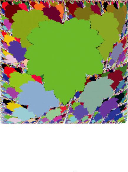
A vast range of tilings and orbital pictures is possible within projective geometry. This is demonstrated in tiny measure by the projective IFS objects illustrated in this book. An orbital picture that is clearly projective is shown in Figure 3.76.

Mobius¨ geometry

The Mobius¨ geometry, GMobius¨, is defined by the group of Mobius¨ transformations acting on the extended complex plane. These transformations are discussed in Chapter 2. They take the form

Figure 3.76 Example of a projective orbital picture. Compare it with the Mobius¨ orbital picture in Figure 3.82 and the affine orbital picture in Figure 3.42.

where a, b, c, d C and ad − bc =0. In this geometry generalized circles are mapped to generalized circles. Angles between intersecting circular arcs are preserved both in magnitude and orientation.

Inversive geometry, Ginversive, is defined by the smallest group of transformations on C that includes the reflection R(z) = z; that is,

Ginversive = GMobius¨ {M ◦ R : M GMobius¨}.

Inversive geometry does not have the property of oriented angles but does admit generalized circles and the magnitude of angles. Euclidean distance is not preserved.

Two-dimensional hyperbolic geometry may be represented by the subgroup of inversive geometry that maps the unit disk D C, centred at the origin, onto

itself. The corresponding Mobius¨ transformations M : D → D are defined by

az + b

¯ + bz a¯

for all z D,

where a, b C with |b| < a.

Hyperbolic geometry was one of the most momentous mathematical discoveries of the nineteenth century; see [25], p. 261. It provided a two-dimensional geometry in which, given any line L and any point P not on L, there exist infinitely many lines through P that do not meet L. For more than two thousand years, since Euclid wrote his famous geometry books, generation after generation of mathematical thinkers asserted that this could not be true in the real physical world. They thought that the only possible geometry for physical space was euclidean geometry. Now hyperbolic geometry is considered as one of various possible models for the space in which the universe is located.

Tilings of the unit disk D associated with hyperbolic geometry, generated by various IFS groups, were popularized by the artist M. C. Escher; see for example [86]. Escher was fascinated by the different ways in which space could be cut up, methodically, into related shapes, reminiscent of animals, people and plants; his paintings suggest that there is something mysterious in geometrical transformations of shape and form. Escher was an artistic explorer, seeking visual geometrical properties of euclidean, Mobius¨ and other geometries.

In effect, some of Escher’s works exploit the fact that there are infinitely many fundamentally different tilings of the unit disk by generalized triangles. A generalized triangle is a three-sided figure whose sides are arcs of generalized circles. This is in striking contrast to the mere seventeen fundamentally different tilings allowed by euclidean geometry.

E x e r c i s e 3.7.16 Type the phrase ‘hyperbolic tilings’ into Google or another internet search utility. Print out some pictures of hyperbolic tilings. Find the corresponding IFS groups.

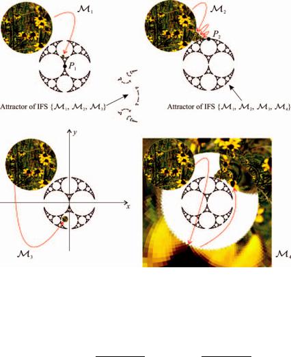
Figure 3.77 This illustrates the action of each of the four Mobius¨ transformations in the IFS in Equation (3.7.1). It shows the result of applying each of these parabolic transformations to the condensation picture used in Figure 3.80, and the relationship to the limit set. The points P1 and P2 denote the fixed points of M1 and M2 respectively.

and the modular group Gmodular(C) , which is associated with the IFS

The four transformations M1(z), M2(z), M3(z), M4(z) GSierpinski(C) are parabolic; it may be helpful here to look back at Figure 2.34. Their actions are illustrated in Figure 3.77. For M1(z) GSierpinski(C), the fixed point is z = 0 and the fixed line is the imaginary axis. This transformation sweeps points lying in the left half-plane in a clockwise direction. The inverse, M3(z) = M−1 1(z) GSierpinski(C), has the same fixed point and fixed line as M1(z) but the orientation of the sweep-

ing motion is opposite. For the parabolic transformation M2(z) GSierpinski(C), the fixed point is z = i and the fixed line is {z C : z = x + i, x R {∞}}.

Points lying above the fixed line are swept in an anticlockwise direction.

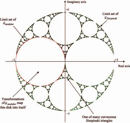
Figure 3.78 Illustration of the relationship between Gmodular and GSierpisnki, defined by the IFSs in Equations (3.7.2) and (3.7.1). The limit set of GSierpisnki is shown in black while the limit set of Gmodular is the red circle.

Gmodular is a subgroup of GSierpisnki.

The relationship between the limit sets of GSierpinski(C) and Gmodular(C) is illustrated in Figure 3.78. These limit sets were computed using random iteration. We chose to represent the modular group using transformations that map the circle centred at − 12 i, of radius 12 , onto itself. The standard representation is obtained by conjugating the transformations here by a Mobius¨ transformation that takes this circle to the upper half-plane. The modular group and its subgroups play an important role in the theory of continued fractions and number theory; see for example [73].

In the sequence of pictures (i)–(vi) in Figure 3.79 we illustrate the panels of a one-parameter family of orbital pictures associated with GSierpinski(C). In each picture, the domain of the condensation picture, shown in black, is the exterior of a circle centred at the origin; the radius R of this circle is decreased successively from R = 2 to R = 1, so that in effect we are zooming in on the circular region

Figure 3.79 Panels of a family of orbital pictures generated by an IFS group of Mobius¨ transformations. In each case the condensation picture, shown in black, is the exterior of a circle centred at the origin, of decreasing radius, although this is masked by the continual zoom in towards the centre. The panels have been given different colours to distinguish them. In the last image, (vi), many panels have merged.

while its radius decreases. In (vi) R = 1 and the circle coincides with the outer boundary of the limit set of the group. In each picture the viewing window is {z = x + i y C : −R ≤ x ≤ R, −R ≤ y ≤ R}. The panels are rendered in various colours. Inside each bubble of the limit set in which there is a panel, there is one disk-shaped panel and many crescent-shaped ‘children’. As R decreases towards 1, the disk-shaped bubble approaches filling up the whole bubble and the children become like waning crescent moons; at R = 1 a quite famous type of picture, associated with the modular group, appears.

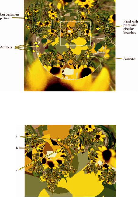
An example of an orbital picture associated with GSierpinski(C) is illustrated in Figures 3.80 and 3.81. Figure 3.81 shows a magnification of part of Figure 3.80 to reveal some structures associated with limiting pictures. The sequences of panels labelled a, b and c correspond to distinctly different limiting pictures.

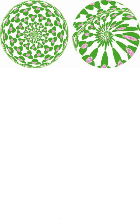
Examples of panels of orbital pictures associated with Gmodular(C) are shown in the right-hand images in Figures 3.82 and 3.83. In each figure the left-hand image