Ohrimenko+ / Barnsley. Superfractals

Figure 4.39 The tops dynamical system and the branches of its inverse, which define a restricted IFS.

The idea of a directed IFS is new to fractal geometry. But a more general structure, of iterated set maps, has been investigated in [69] and is quite closely related.

4.17The top of a directed IFS

The following will tell us that most of the theory of transformations between fractal tops goes through for directed IFSs. Hence lies our success in colour-stealing, using directed IFSs in place of hyperbolic IFS, as illustrated in Figure 4.37. The main difference, in general, is that there is no tops dynamical system.

We present the main ideas somewhat concisely, and in such a way that they can be used in Chapter 5 in connection with superfractals. These key ideas are the same as in Section 4.14, and the proofs, which we omit, are entirely analogous. I want to stress here that although these ideas are very simple, they may look complicated because they require quite a few symbols for their expression.

Let F = {X; f1, f2, . . . , fN } be a hyperbolic IFS. Let AF denote its attractor and let φF : {1,2,...,N } → AF denote the associated addressing function. Let{1,2,...,N } be closed and define

A(F, ) = φF ( ).

When is shift invariant, (F, ) is of course a directed IFS and A(F, ) is a deterministic fractal, but we want to discuss sets of the form of A(F, ) quite generally. Indeed, in Chapter 5 we will represent certain V -variable and random fractal sets in just this way. Now let τ(F, ) : A(F, ) → be defined by

τ(F, )(x) = max{σ : φF (σ ) = x} for all x A(F, ).

Notice that

(φF ◦ τ(F,))(x) = x for all x A(F,).

We define the restricted tops code space (F,) to be the set

(F,) := τ(F,) A(F,) = τ(F,)(φF ( ))

and we define

φ(F,) : (F,) → A(F,)

to be the restriction of φF to the closure of (F,). The latter maps the closure of(F,) continuously onto A(F,).

When (F, ) is a directed IFS we call Q(F,) the restricted code structure of the directed IFS (F, ). We remark that clearly on the one hand not all sets possess restricted code structures and on the other hand a set may possess many restricted code structures. Moreover, we may consider ‘projective restricted code structures’ and ‘Mobius¨ restricted code structures’, with obvious meanings; then we discover that projective restricted code structure is a property of projective geometry, and so on, along the lines discussed at the end of Chapter 3.

D e f i n i t i o n 4.17.2 We say that two restricted code structures Q(F,) and Q(G,) are homeomorphic iff there is a homeomorphism χ : (F,) →(G,) that respects the code structures, that is, such that q Q(F,) χ (q)

Q(G,).

T h e o r e m 4.17.3 Let the two restricted code structures Q(F,) and Q(G,) be homeomorphic. Then A(F,) and A(G,) are homeomorphic. That is, there exists a homeomorphism H : A(F,) → B(G,) such that

H A(F,) = A(G,).

If the homeomorphism χ : (F,) → (G,) has the property that χ ( (F,)) =(G,) then

τ(G,) ◦ H = χ ◦ τ(F,).

P r o o f This follows similar lines to the discussion in Section 4.14 and is therefore omitted.

Analogous results to those concerning fractal transformations apply to directed IFSs and, as we will see in Chapter 5, in connection with superfractals. This extends our ability to construct homeomorphisms between pictures and between objects. One immediate application is to the construction of synthetic imagery

via colour-stealing plus tops, where now ‘tops’ has a more general meaning. (For example, the continuous deformations between the pictures in Figure 5.13 rely on Theorem 4.17.3.)

4.18A very special case: S : → is open

Here we quote the brilliant work of William Parry, showing that a directed IFS is essentially a graph-directed IFS if and only if S : → is open.

We consider the symbolic dynamical system S : → where {1,2,...,N } is a closed set with S( ) = . The topology on is the restriction of the natural topology on {1,2,...,N } to . Equivalently, the topology on is the natural topology of the compact metric space (, d ). See Theorem 1.9.6.

Recall that a cylinder set of {1,2,...,N } is a subset of {1,2,...,N } that can be written in the form

C(σ ) := ω {1,2,...,N } : ωn = σn for all n = 1, 2, . . . , |σ | ,

for some σ {1,2,...,N }. A set C is called a cylinder set of when it is the same as the intersection of a cylinder set of {1,2,...,N } with ; that is, when

there exists a cylinder set C {1,2,...,N } such that C = C ∩ . Let us introduce the notation

:= σ {1,2,...,N } : C(σ ) ∩ = { }.

That is, consists of the set of all finite-length ‘beginnings’ of strings which belong to , together with the empty string. An important property of is that its cylinders are both open and closed. The transformation S : → is continuous, but it is not necessarily open, as illustrated at the end of Section 4.16.

Parry [77] defines the dynamical system S : → to be an intrinsic Markov chain of order r when the following condition is satisfied: whenever k is a positive integer with k ≥ r , then

T h e o r e m 4.18.1 Let {1,2,...,N } be closed and shift invariant. Then the dynamical system S : → is an intrinsic Markov chain iff S is open.

In the course of his proof, Parry shows that the pair of equivalent assertions in the statement of the theorem are also equivalent to the following: there exists a finite set of cylinders {C(σ (m)) : m = 1, 2, . . . , M}, where σ (m) and

This is equivalent, back on the attractor A of the directed IFS, to the statement

kind that, in essence, underlies recurrent IFSs, see [10], and graph-directed IFSs, as described in [68] and [98]. This shows that the concept of directed IFSs subsumes these other well-known generalizations of IFS theory.

4.19Invariant measures for tops dynamical systems

Here, most briefly, we alert the reader to the rich literature that exists regarding invariant measures associated with symbolic dynamical systems. In the case where the system derives from a fractal top, the tops dynamical system and the corresponding symbolic dynamical system are often equivalent, and invariant measures that assign zero to each single point can be moved painlessly back and forth between the two systems. These measures are relevant to the design of efficient algorithms for computing tops functions; the question when such measures have maximum entropy, or are nice and smoothly distributed on the fractal top, is very interesting. In this regard we note the work of Lasota and Yorke [61] and more recent studies that cite it.

We are interested in normalized Borel measures defined on the Borel field generated by the cylinders of . Quite generally, given any closed shift-invariant code space {1,2,...,N } there exists at least one measure μ P( ) such that S(μ) = μ; see [56], p. 139.

The symbolic dynamical system S : → is called regionally transitive iff, whenever σ and ω belong to , there exists an integer n such that

S◦n (C(σ )) ∩ C(ω) = .

We quote the following from [77], p. 371.

T h e o r e m 4.19.1 If S : → is a regionally transitive symbolic dynamical system then there is a normalized Borel invariant measure μ, with respect to which S is ergodic, such that

hμ(S) = e(S),

By means of the tops transformation, we can use such measures to define corresponding invariant measures for corresponding tops dynamical systems. These are relevant to the efficient computation of fractal tops with algorithms that are of the chaos game type. We note the recent review by Zbigniew Nitecki [75] on the topological entropy and pre-image structure of symbolic dynamical systems.

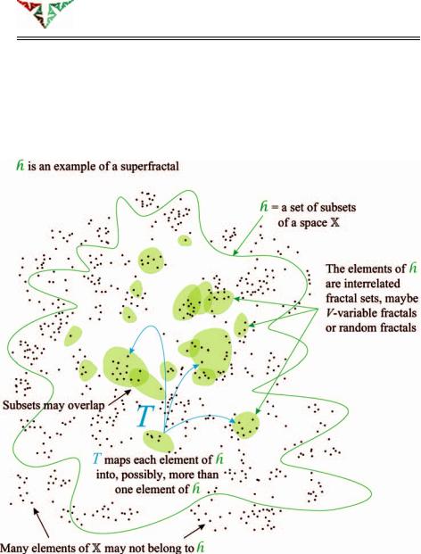
Figure 5.1 A superfractal of seascapes is represented here by diverse triangular pictures surrounding the square ocean picture. The triangular pictures correspond to samples of a particular superfractal, produced by the chaos game. See the text for more details.

of ideas from all of us we soon had superfactals up and running on a computer, and we realized that they were significant and, in the case V ≥ 2, new. The important case of ‘1-variable’ sets is a special case of a type of random fractal investigated by Kifer and others; see [43], [3], [59] and [90]. See also [2]. The computational experiment described below in Section 5.2 was in essence the first experiment we ran. The basic theory of V -variable sets and measures and some applications first appeared in [16], which is the main source for the presentation here. Subsequent developments are reported in [19], [20] and [21]; see the end of Section 5.19.

5.2 Computational experiment: glimpse of a superfractal

We begin by describing a computational experiment that gives you the basic idea of how to compute V -variable fractals. This experiment was first described in published form in [16]. We start with two projective IFSs, F1 = { ; f11, f21} and F2 = { ; f12, f22}, where := [0, 1] × [0, 1] R2. The IFS codes are given in Tables 5.1 and 5.2.

In Figure 5.3 we illustrate the action of F1 and F2 on a triangle ABC. Both F1 and F2 are linked IFSs, and their attractors, pictures of which are included

Table 5.1 Projective IFS code for one of the two IFSs used in the computational experiment. The attractor is pictured below, as in the tables that follow. See Figure 5.3

Figure 5.2 Illustation of some aspects of a superfractal. See also Figure 5.22. The transformation T is explained in Section 5.18.

Table 5.2 The other IFS code used in the computational experiment

Figure 5.3 The actions of the two affine IFSs F1 (upper arrows) and F2 (lower arrows) used in the computational experiment.

in Figure 5.6, may be represented as the graphs of continuous mappings gm : [0, 1] → R2, m = 1, 2, such that g1(0) = g2(0) and g1(1) = g2(1). We say that these continuous paths are tethered at A and C.

To set up the experiment we need two pairs of digital buffers, i.e. memory displays, ( 1, 2) and ( 1 , 2 ). Each buffer is the same size and may be used to represent binary, black-and-white, images. The buffers are discretized copies ofR2. The value 0 is assigned to white pixels and the value 1 is assigned to black pixels. We refer to these pairs of buffers as the input screens and output screens respectively. We also need a digital processor that can read from and write to each pair of buffers.

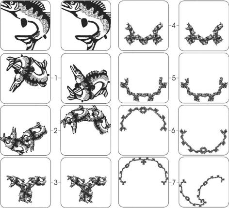
We initialize the experiment by setting some of the pixels to 0 and some to 1 on each input screen, as illustrated by the two fish in the top pair of images on the left in Figure 5.4. We also clear both output screens by setting all their pixels to zero.

Figure 5.4 Shows successive pairs of images produced in the course of the computational experiment described in Section 5.2.

We now construct a sequence of pairs of images, which appear successively in pairs on the output screens, as follows.

(i)Pick randomly one of the IFSs F1 and F2, say Fn1 . Apply f1n1 to the image on either 1 or 2, selected randomly, to make an image on 1 . Then apply f2n1 to the image on either 1 or 2, also selected randomly, and overlay the resulting image I on the image now already on 1 . That is, form the union of the black region of I with the black region on 1 and put the result back onto 1 .

(ii)Again pick randomly one of the IFSs F1 and F2, say Fn2 . Apply f1n2 to the image on either 1 or 2, selected randomly, to make an image on 2 . Also apply f2n2 to the image on 1 or 2, also selected randomly, and overlay the resulting image on the image now already on 2 .

(iii)Switch input and output, clear the new output screens and repeat steps (i) and (ii).