Ohrimenko+ / Barnsley. Superfractals

4.16 Directed IFSs and general deterministic fractals

Here we introduce a natural generalization of the IFS concept called a directed IFS. The basic idea is very simple and has the virtue of being easy to understand and apply.

This is not generalization for its own sake! Firstly we will show that there exists a unique attractor that obeys a self-referential equation; thus we obtain a wider class of deterministic fractals. Secondly, the concept of a directed IFS handles multiple fractals simultaneously and is such that the theory of fractal tops and fractal homeomorphisms, adjusted to the more general setting, continues to hold. This means that we can deal topologically with multiple set attractors within a single coordinate system. Thirdly, the directed IFS framework subsumes the other main generalizations of the IFS framework, including deterministic graphdirected IFSs [68], recurrent IFSs [10] and local IFS theory [12]. Fourthly, this generalization arose in an entirely natural manner upon consideration of fractal tops and of the boundaries of set attractors of IFSs: how might one describe the essential features of a fractal top without having to go through all the usual IFS machinery?

In this brief introduction to directed IFSs we concentrate on aspects related to set attractors and fractal tops. We leave it to the reader to apply the same underlying idea to generalize orbital pictures, orbital sets, orbital measures and so on, as needed.

Let F denote a hyperbolic IFS, with attractor A, code space and code space mapping φF : → A. Let 0 denote any shift-invariant subspace of code space, and let 0 be closed. A shift-invariant subspace is one that is unchanged by the application of the shift transformation S : → . So we have

S : → , 0 , S| 0 : 0 → 0 and S| 0 ( 0) = 0.

D e f i n i t i o n 4.16.1 A directed IFS is an IFS F = {X; f1, f2, . . . , fN } together with a closed nonempty shift-invariant subspace 0 = {1,2,...,N }. It is denoted by (F, 0) or by

({X; f1, f2, . . . , fN }, 0).

For simplicity we assume throughout that X is a compact metric space and that F is hyperbolic.

D e f i n i t i o n 4.16.2 The set attractor of the directed IFS (F, 0) is the set

A0 = φF ( 0).

We think of the order in which the functions in the IFS may be applied as being ‘directed’ by the shift-invariant subspace 0. This is distinct from a

graph-directed IFS, where the order in which the functions may be applied is restricted to orderings specified by a (combinatorial) graph. It follows easily from the above definitions that the set attractor of a directed IFS (F, 0) is a compact subset of the set attractor of F. Think no less of it for that. After all, consider how many interesting compact sets there are in the filled unit square!

The following theorem tells us that a compact set obeys a self-referential equation of a very general kind, Equation (4.5.11), iff it is the set attractor of a directed IFS.

T h e o r e m 4.16.3 Let F = {X; f1, f2, . . . , fN } be a hyperbolic IFS, and let φF : {1,2,...,N } → AF denote the corresponding code space mapping. Then there exist compact sets An X for n = 1, 2, . . . , N , at least one of which is nonempty, such that

A1 A2 · · · AN = f1( A1) f2( A2) · · · fN ( AN ) (4.16.1)

iff there is a closed set 0 {1,2,...,N } such that (F, 0) is a directed IFS whose set attractor is A0 = A1 A2 · · · AN .

P r o o f Suppose that ({X; f1, f2, . . . , fN }, 0) is a directed IFS whose attractor is A0 X. Then

A0 = φF ( 0) = φF ( 1) φF ( 2) · · · φF ( N ),

where n = {σ 0 : σ1 = n} for n = 1, 2, . . . , N . But this is the same as

A0 = f1 φF (S( 1)) f2 φF (S( 2)) · · · fN φF (S( N )) . So, we define An = φF (S( n )). Then we have

A0 = f1( A1) f2( A2) · · · fN ( AN ).

But the shift invariance of 0 implies that

0 = S( 0) = S( 1 2 · · · N ) = S( 1) S( 2) · · · S( N ),

which provides us with

A0 = φF ( 0) = φF (S( 1)) φF (S( 2)) · · · φF (S( N )

= A1 A2 · · · AN .

Since φF and S are continuous and 0 is compact and nonempty, it follows that the sets A1, A2, . . . , AN are compact and at least one of them is nonempty.

Conversely, suppose that there exist compact sets An X for n = 1, 2, . . . , N such that

A1 A2 · · · AN = f1( A1) f2( A2) · · · fN ( AN ).

372 Hyperbolic IFSs, attractors and fractal tops

Let x1 f1( A1) f2( A2) · · · fN ( AN ). Then there exist σ1 {1, 2, . . . , N } and x2 Aσ1 such that fσ1 (x2) = x1. But then x2 f1( A1) f2( A2) · · · fN ( AN ), so there exist σ2 {1, 2, . . . , N } and x3 Aσ1 such that fσ2 (x3) = x2. Continuing in this manner we find a sequence of σk s and xk s such that

x1 = fσ1 ◦ fσ2 ◦ · · · ◦ fσk (xk+1).

But the sequence on the right converges to φF (σ ), where σ = σ1σ2 · · · . It follows that we can find a subset 0 of code space such that φF ( 0). This subset can be chosen to be closed and shift invariant. The latter is immediate and the former is achieved by taking the closure of 0 in case it is not already closed. Finally, 0 is nonempty because at least one An is nonempty.

In view of Theorem 4.16.3 and the content of Theorems 4.16.6 and 4.16.7 below, and of Section 4.17, we make the following definition. The concept of a directed IFS is a convenient theoretical structure for handling the diverse properties of all sets that, it appears to me, it is natural to call ‘deterministic fractals’.

D e f i n i t i o n 4.16.4 A compact nonempty subset A0 of a complete metric space X is called a deterministic fractal (set) iff there are nonempty compact

Why do we call these objects ‘fractals’? The set attractor of an overlapping IFS has the same dimension as the space in which it lies, say R2. We call the set attractors of directed IFSs ‘fractal’ because they possess distinctive subsets, such as their boundaries, that do indeed appear typically to possess non-integer Hausdorff dimension.

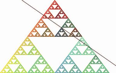
As a simple example of a directed IFS let F1 = {R2; f1, f2} have attractor A1. Let

F2 = {R2; f3, f4, f5}

have attractor A2 that intersects A1. For example see Figure 4.34, where A1 is a Sierpinski triangle and A2 is a line segment. Let

0 = {1,2} {3,4,5} {1,2,3,4,5}.

Then it is readily verified that 0 is shift invariant and that

A0 = A1 A2.

So here the attractor of a directed IFS is the union of the attractors of two IFSs. This might all seem rather trivial. But it is not. As we will show in Section 4.17, the theory of fractal tops and related homeomorphisms can be adapted to directed IFSs: two deterministic fractals have the same code structure iff they are homeomorphic. This means that we can handle multiple fractals and their intersections, using

Figure 4.34 The natural topology of A 1 A 2 is the same as the identification topology induced by φ0 : 0 → A 0. Here A 1 is a Sierpinski triangle and A 2 is a line segment.

code space manipulation, in ways that are somewhat analogous to the handling of intersections of geometrical objects such as parabolas and straight lines using coordinate geometry. But our conclusions will of course be topological rather than geometrical!

The next simple examples show that the attractors of directed IFSs may be much more complicated. Let

0 = σ {1,2,...,5} : σk {1, 2, 4} σk+1 {1, 2, 3},

otherwise σk+1 {4, 5}, for all k .

Then it is easy to see that, by the very form of its definition, 0 = S( 0). Let

F1 = R2; 12 (x + 2), 12 (y + 1) , 12 (x + 3), 12 y ,

12 (x + 4), 12 y , (x − 2, y), (−x + 1, −y + 1) .

Then the set attractor of the directed IFS (F1, 0) is precisely the set pictured in Figure 0.6 in the Introduction, consisting of a triangle and a square. Look back and see how the chaos game was used to compute this set attractor. Let

0 = σ1σ2 · · · σk : σ 0, k {0, 1, . . . } .

Then you will see that at the kth step of the chaos game we generate a string σ 0 of length k and compute the point fσ (x0). Clearly these approximations approach elements of A0 geometrically fast, and distribute themselves ergodically upon it, in the usual manner. In Figure 4.35 we show a decomposition of A0 into sets A1, A2, A3, A4 and A5, corresponding to Equation (4.16.1).

Figure 4.35 The upper two images show the set attractor A 0 of the directed IFS (F1, 0) and the sets A 1, A 2, A 3, A 4 and A 5 in the self-referential Equation (4.16.1). The lower two images show how A 0 is the union of f1( A 1), f2( A 2), f3( A 3), f4( A 4) and f5( A 5).

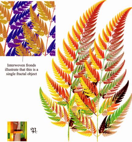
Two related examples are illustrated in Figures 4.36 and 4.37. In Tables 4.9 and 4.10 we give the IFS codes for the set of projective transformations described in Figure 4.38. Note that neither IFS on its own makes a fern! The IFS in Table 4.9 represents a ‘fern’ in which the fronds do not meet the main stem, while the IFS in Table 4.10 represents a ‘fern’ in which the stalks of the fronds stick out of the opposite side of the main stem. Here we choose the IFS to be {R2; f1, f2, . . . , f8}. But we choose the shift-invariant space to be

0 = σ {1,2,...,8} : σk {1, 2, 3, 4} σk+1 {1, 2, 7, 8},

otherwise σk+1 {3, 4, 5, 6}, for all k .

It is readily verified that S( 0) = 0. In fact, if we write 0 = 1 + 2, where

1 = {σ 0 : σ1 {1, 2, 7, 8}}

and

2 = {σ 0 : σ1 {3, 4, 5, 6}},

then the two individual ferns, which appear superimposed in Figure 4.37, are given by φF ( 1) and φF ( 2), and we note that S( 1) = S( 2) = 0.

How do we know that the above description is correct? Really, this follows from noting that these examples can be re-expressed in the language of recurrent

Figure 4.36 The two main images constitute a single set attractor of a directed IFS, but neither fern on its own is an attractor. It has been coloured by colour-stealing from the picture PC shown inset.

IFS theory; see [10] or [13]. But many shift-invariant subspaces do not correspond to finite-order Markov processes, as will be explained in Section 4.18.

We will use the following definition several times in the next few pages.

D e f i n i t i o n 4.16.5 Let X and Y be topological spaces. A transformation f : X → Y is called open iff f (O) is open whenever O X is open.

The following theorem says that the boundary of the set attractor of an IFS may contain an interesting deterministic fractal, provided that all the transformations involved are open.

T h e o r e m 4.16.6 Let F = {X; f1, F2, . . . , fN } be an IFS such that each transformation fn is open. Let A denote the set attractor of F and let ∂ A denote

Figure 4.37 A recurrent IFS, corresponding to the eight transformations in Tables 4.9 and 4.10, generated this single attractor (main figure). This is a picture of the fractal top of this directed IFS, computed using the chaos game. The panel at top left shows the intricate interplay of the object with itself. The picture PC from which colours were stolen is shown inset.

its boundary. Then there exist closed subsets ∂ An ∂ A such that

∂ A = f1(∂ A1) f2(∂ A2) · · · fN (∂ AN ).

Let φF : → A denote the code space function associated with F. If ∂ A is nonempty and 0 = φF−1(∂ A) then S( 0) 0 and consequently 0 contains a closed nonempty shift-invariant subset 0 = lim S◦k ( 0). The attractor of the

k→∞

directed IFS (F, 0) is contained in ∂ A.

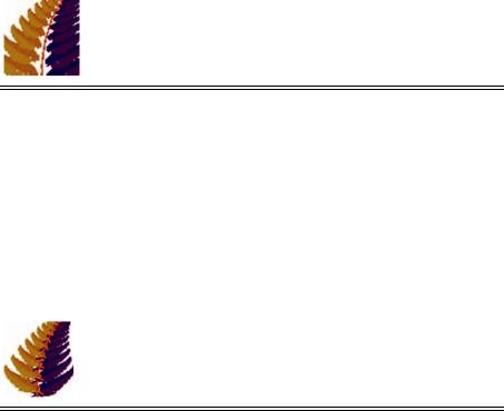
Table 4.9 A projective IFS code. This, together with the code in Table 4.10, is used in Figure 4.37. Part of the attractor is shown below. A similar but different pair of IFS codes was used to produce Figure 4.36

Table 4.10 A projective IFS code. Part of the attractor is pictured below. This code, together with the values in Table 4.9, is used in Figure 4.37

In the last step here we have used the fact that the transformations fn are open. It now follows that no point in the boundary of A is the image under any fn of a point in the interior of A. Hence each point on the boundary must be the image of a point on the boundary under one of the fn . This proves the first assertion. It also follows that S( 0) 0. Consequently {S◦k ( 0)}∞k=1 is a nested sequence of nonempty compact sets which converges to a nonempty compact set 0 such that S( 0) = 0. The attractor of the directed IFS (F, 0), namely φF ( 0), is clearly contained in ∂ A. I have drawn attention to this special subset of the boundary of the attractor of F because I think it is the key to understanding the boundary as a whole; it may be treated as a condensation set from which

Figure 4.38 The actions of the eight transformations, given in Tables 4.9 and 4.10, of the directed IFS used in Figure 4.37 are illustrated here by showing how they act on leaf-shaped regions corresponding to the whole or part of the ferns in Figure 4.37.

the whole boundary may be constructed, quite naturally, by iterated application

Local IFSs are used extensively in fractal image compression, see [12], and there are efficient algorithms for computing their attractors, including pixel-chaining; see for example [62], pp. 207–10. The latter can be readily adapted to the

computation of the ‘top’ of the attractor of a local IFS. We mention local IFSs here because they provide a rich source of deterministic fractals.

T h e o r e m 4.16.7 Let F = {X; fn : Xn → X, n = 1, 2, . . . , N } be a local IFS. Then it possesses at least one attractor A. Each attractor of a local IFS is a deterministic fractal.

P r o o f Define K0 = X and, recursively,

Kk = f1(X1 ∩ Kk−1) f2(X2 ∩ Kk−1) · · · fN (XN ∩ Kk−1)

for k = 1, 2, . . . Then the sequence of sets {Kk H(X)}∞k=0 is a decreasing sequence of compact sets and so possesses a unique limit A. This limit obeys Equation (4.16.2). Let An = Xn ∩ A. Then

Note that the union of two attractors of a local IFS is also an attractor. In particular, a local IFS possesses a unique ‘largest’ attractor, that mentioned in the proof of Theorem 4.16.7 above.

A rich class of directed IFSs is provided by fractal tops. If F is the tops

code space of a hyperbolic IFS F then F is shift invariant and (F, F ) is a directed IFS. Its set attractor is the same as the set attractor of F. Typically, when the IFS F is overlapping, the symbolic dynamical system formed by the shift transformation acting on the closure of the tops code space, S : F → F , does

not correspond to any finite-order Markov chain, because the mapping S : F →F is not open. This means that techniques used to explore invariant measures and attractors associated with recurrent IFSs [10] and graph-directed IFSs [68] may not be generally applicable to directed IFSs.

A specific example is provided by

F = {[0, 1] R; f1(x) = β x + (1 − β), f2(x) = αx},

where 0.5 < α < 1, 0.5 < β < 1, and is illustrated in Figure 4.39. We find that

It is possible to establish many cases for which τF ((1 − β)/α) does not end in 1, for example if we choose α = β = 2/3. Then S : F → F is not open. See [77].