Ohrimenko+ / Barnsley. Superfractals

Figure 4.23 Illustrates the domains D1, D2, D3, D4 for the tops dynamical system associated with the IFS given used to make Figure 4.16. Once this ‘picture’ has been computed it is easy then to compute the tops function. Just follow the orbits of the tops dynamical system!

for all x A. Moreover, ξ P(X) is an invariant probability measure for { A, T } iff τ (ξ ) P( ) is an invariant probability measure for { τ , S}.

P r o o f This follows directly from everything we have said above. But do not confuse an invariant measure ξ P(X) of T , which obeys ξ = T (ξ ), with the unique measure attractor μ P(X) of F, which obeys μ = F(μ). Compare with Theorem 4.9.3.

In the special case where the IFS is totally disconnected and the fn are one-to- one then T : A → A is defined by T (x) = fn−1(x), where n is the unique index such that x fn ( A). This dynamical system has been considered elsewhere, for example in [14], [4] and [58]. It is interesting because in this case φ : → A is a homeomorphism and T is conjugate to the shift transformation on code space, according to

T = φ ◦ S ◦ φ−1.

We see that in this case τ = φ−1. In this special case the topological entropy of T is log2 N .

C o r o l l a r y 4.11.4 The value of τ (x) may be computed by following the

orbit of x A as follows. Let x1 = x and xk+1 = T (xk ) for k = 1, 2, . . . , so that the orbit of x is {xk }∞k=1. Then τ (x) = σ where σk {0, 1, . . . , N − 1} is the unique index such that xk Dk for all k = 1, 2, . . .

P r o o f This follows directly from Theorem 4.11.3. At the risk of being repetitive, notice the following points. (i) The IFS F has totally disconnected

all y A. The key observation is that the orbit of a point on the top stays on the top, and so the code given by its orbit is the value of the tops function applied to the point.

The following theorem explains precisely what we mean when we say that tops

=

where ∂ Dn denotes the boundary of Dn , as defined in Equation (4.11.1). Then the restricted tops dynamical system T |Ainside : Ainside → Ainside is continuous. Also, the restricted tops function τ |Ainside : Ainside → is continuous.

Here and elsewhere we use the notation T ◦(−k)(S) (i.e. T −1 composed with

Then, since each of the functions T ◦k (x) is continuous on Ainside, we can find δ > 0 such that T ◦k (y) belongs to the interior of Dσk for k = 0, 1, . . . , M whenever d(x, y) < δ. It follows from Corollary 4.11.4 that τ (y) agrees with τ (x)

352 Hyperbolic IFSs, attractors and fractal tops

through the first M symbols, that is, (τ (y))k = (τ (x))k = σk for k = 0, 1, . . . , M

E x e r c i s e 4.11.6 Show that the tops dynamical system for the IFS F1 in Equation (4.9.1) is correctly defined by Equation (4.14.2) and correctly illustrated in Figure 4.27. (This dynamical system is closely related to the one studied by A. Renyi [82] in connection with information theory. The IFS F1 also appears in the context of Bernoulli convolutions; quite recently, a longstanding problem regarding the absolute continuity or otherwise of the measure attractor of F1 was solved by Boris Solomyak; see [89].)

E x e r c i s e 4.11.7 Look up ‘Markov partitions’ on the internet. Important research publications in this general area have been written by David Ruelle, Y. G. Sinai, Rufus Bowen, Caroline Series, Brian Marcus and many others. What are the objectives of research in symbolic dynamics?

4.12The fractal top is the fixed point of FTOP

Next we show that τ (x) is the unique fixed point of a contractive transformation, closely related to F : (X) → (X). Here we take = {1,2,...,N }{1,2,...,N }. We recall, from Section 1.6, that ( , d ) is a compact metric space.

We define FTOP : (X) → (X) as follows. Let P (X), and let DP denote the domain of P. Then we define the set of disjoint sets by

D1 = f1(DP),

D2 = f2(DP)\D1,

D3 = f3(DP)\(D1 D2),

.

.

.

DN = fN (DP)\(D1 D2 · · · DN −1).

Let the domain of FTOP(P) be D1 D2 · · · DN , which is the same as the

Let ( A) ( A) (X) denote the set of functions with domain A and range in . Then it is easy to see that FTOP( ( A)) ( A). Also, you can readily check that ( ( A), dsup) is a complete metric space with respect to the distance function

dsup(P1, P2) = sup d (P1(x), P2(x)).

x A

T h e o r e m 4.12.1 Let F be a hyperbolic IFS of invertible transformations, and let FTOP : ( A) → ( A) denote the restriction of FTOP, as defined above, to ( A). Then FTOP is a contraction mapping, with contractivity factor 0.5, on the complete metric space ( ( A), dsup). Its unique fixed point is τ , the tops function of F.

= (0.5)dsup(P1, P2).

It remains to verify that FTOP(τ ) = τ . Suppose that x Dn = fn ( A)\ f1( A)

· · · fn−1( A). Then, by definition,

Consequently we can obtain a deterministic sequence {τk (x)}∞k=0 of approximations to the tops function τ (x) by starting from any function τ0 : A → and iteratively defining

τk+1(x) = (FTOP(τk ))(x) for k = 0, 1, 2, . . . ,

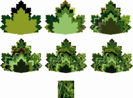
for all x A. An example is illustrated in Figure 4.24. This is based on the same IFS as used in Figure 4.11, where we encountered the texture effect. In this example we took τ0 ( A) to be a constant,

τ0(x) = σ (0) {1,2,3,4} for all x A

where σ (0) = 1. It is easy to see that in this case we have τk : A → {1,2,3,4} rather than τk : A → {1,2,3,4} {1,2,3,4}. This allows us to represent the approximant τk by colouring its graph using colour-stealing, that is, by rendering the point x A in the colour PC (φD (τk (x))). The picture PC is a digital photograph of some grasses, shown at the bottom of Figure 4.24. In contrast with the situation in Figure 4.11, this sequence of pictures converges to a stable (no visible texture effect) picture, despite discretization errors, after about sixteen iterations. That is, rendered to viewing resolution, PC (φD (τ16)) = PC (φD (τ17)) = · · · To check our

Figure 4.24 This illustrates a sequence of six pictures converging to the unique fixed point of the fractal tops operator FTOP. From left to right, the first, second, third, fourth, eighth and thirteenth iterations are shown. At the printed resolution, the image ceases to change with further iterations. The picture from which the colours were stolen is at the bottom. See the main text. No texture effect here!

results, we used a coupled chaos game to compute PC (φD (τ )) and found the same picture.

So now it is possible to see how the texture effect, and the general lack of ‘closure’ that we first noticed in connection with orbital pictures and underneath pictures, led to the discovery of fractal tops!

4.13 Relationship between fractal tops and some orbital pictures

To get a feel for what will be discussed in this section, look back at Figures 3.32, 3.49 and 3.50. The idea, formalized below, is that in some cases the set of accumulation points of the addresses of the panels in an orbital picture, P0 , is equal to the closure of τ . Consider the family of IFSs

parameterized by λ (0, 1). This is similar in spirit to the family of IFSs in Equation (3.5.17), which was used to generate Figure 3.32. Let P0 be a picture whose domain is the line segment that joins the two points (0, 1) and (1, 1) in ,

4.13 Relationship between fractal tops and some orbital pictures 355

Figure 4.25 Here some panels of an orbital picture P(P0) are labelled with their addresses. Each labelled line segment F◦k (P0) defines an approximation τk (x ) to the top τ (x ) of the IFS F in Equation (4.13.1) with λ = 0.25. The attractor of the IFS is the line segment [0, 1] contained in the x -axis. In such examples

P0 = τ .

namely the upper pair of corners of . The first few generations of panels and their addresses are illustrated in Figure 4.25. Let [0, 1] × 2−k denote the line segment that joins the pair of points (0, 2−k ) R2 and (1, 2−k ) R2, for k = 1, 2, . . . Then the domain of the orbital picture P(P0) is the union of these line segments, and we can define a piecewise constant function τk (x) whose value is the address of the

panel to which (x, 2−k ) belongs. In this case we recognize that τk (x) = FTOP◦k (τ0(x)) where τ0(x) = for all x [0, 1]. But [0, 1] is the set attractor of F and so, by

Theorem 4.12.1, {τk (x)}∞k=0 converges to τ (x). In particular, as proved in Theorem 4.13.1 below, the set of accumulation points of the set of addresses of all the panels here, that is, the set P0 , is the same as the closure of τ .

Next we generalize this example. This provides a link between some orbital pictures and tops functions. Many other specific results connecting P0 and τ can be obtained in a similar vein, but we do not have a more general simple theorem.

Let F = {X; f1, f2, . . . , fN } be a hyperbolic IFS on a compact metric space (X, d). Let A denote the set attractor of F and let τ denote the associated tops code space. Let X = X × [0, 1] and define a metric d on X by d ((x1, x2), (y1, y2)) = d(x1, x2) + |y1 − y2|, so that (X , d ) is a compact metric space. Let F denote

1, 2, . . . , N . Then we look at the orbital picture P (P0) produced when the IFS semigroup generated by F acts on a condensation picture P0 C(P ) with domain

DP0 = A × {1}. Then the domains of (F )◦k (P0), namely

F◦k ( A) × 2−k = A × 2−k for k = 0, 1, 2, . . . , are disjoint, and we have

∞

−k

DP (P0 ) = A × 2 .

k=0

In particular, the union of the domains of the set of panels of P (P0) having code

length k is precisely the set A × {2−k }. Accordingly we can define a function Pk : A → , where = {1,2,...,N }, by

Pk (x) = address of the unique panel of P (P0) whose domain contains (x, 2−k ),

for k = 0, 1, 2, . . . , for all x A. But it will be recognized by the alert reader that

for k = 0, 1, 2, . . . , where we note that P0 ( A) is given by

P0(x) = for all x A.

Now let P0 denote the code space of the orbital picture P (P0).

T h e o r e m 4.13.1 Let τ denote the range of the tops function τ : A → for a hyperbolic IFS F. Let P0 be the set of addresses of the orbital picture P (P0), constructed above. Then

P0 = τ .

P r o o f Suppose that σ P0 . Then there is an infinite strictly increasing sequence of positive integers {kl }l∞=1 such that

σ1σ2 · · · σkl P0

for l = 1, 2, . . . But Equations (4.12.1) and (4.13.2) together imply that

Pk (x) = (τ (x))1(τ (x))2 · · · (τ (x))k for all x A (4.13.3)

and for k = 0, 1, 2, . . . It follows that there exists xkl A such that the first kl symbols in the address τ (xkl ) agree with the first kl symbols in σ . It follows thatτ = τ ( A) contains points arbitrarily close to σ and that σ τ .

Conversely, suppose that σ τ . Then there is a infinite sequence of points

{ω(kl )}l∞=0 in τ such that σ1σ2 · · · σkl ω(kl ) τ for l = 1, 2, . . . Let xkl = τ −1(σ1σ2 · · · σkl ω(kl )). Then, by Equation (4.13.3), Pkl (xkl ) = σ1σ2 · · · σkl . Hence

σ P0 .

In some other cases, such those suggested by Figure 3.43, we have found thatP0 τ . This is interesting because, as described in Theorem 3.5.13, S( P0 )P0 . It suggests that in some cases we can use orbital pictures to probe the structure

of fractal tops and find interesting shift-invariant subsets of τ . We are interested in such shift-invariant subsets because of their association with homeomorphisms between fractals, which we discuss in the remainder of this chapter.

In yet other situations we find that P0 τ , as illustrated in the following exercise.

E x e r c i s e 4.13.2 Let F = { ; (0.75x, 0.5y), (0.75x + 0.25, 0.5y)} and let

P0 ( ) denote the picture whose domain is the point (0.12179 · · · , 1) and whose value is 111111 · · · Consider the associated orbital picture P(P0). Show that if the number 0.12179 · · · is irrational then P0 = {1,2}, τ = {1,2} and, in particular, P0

4.14 The fractal homeomorphism theorem

Sometimes, when looking at different stolen pictures rendered using the same code space picture PC ◦ φC , you will gain the impression that some pairs of them are homeomorphic while others are not. Such is the case with the pictures in Figure 4.26. Look also at Figure 4.2. This shows two colourful fractal ferns, produced by tops plus colour-stealing, corresponding to different IFSs, say FD1 and FD2, but using the same picture PC and the same colouring IFS FC . Here it seems that the underlying attractors are not homeomorphic because, intuitively, any continuous mapping H from one to the other would be forced to identify the set of points where the two lowest fronds join the main stem; thus H would not be invertible. In this way we are led to ask: when are IFS set attractors homeomorphic? Also, when does there exist a one-to-one continuous invertible transformation between one fractal top and another? When are two tops dynamical systems topologically conjugate?

These questions turn out to have a wonderful answer, which is stated formally in Theorems 4.14.5 and 4.14.9 and Corollary 4.14.8 below: roughly, two set attractors are homeomorphic if and only if they can be expressed as the set attractors of two IFSs whose tops code spaces have the same structure up to permutation, regardless of the underlying spaces on which the IFSs act. Also, in this case, their tops functions and tops dynamical systems are topologically conjugate. Of course, we need to explain carefully what we mean by the structure of a tops code space.

Figure 4.26 Which two of these stolen pictures may be related by a continuous invertible deformation? All four pictures of IFS set attractors were rendered using the same mapping, PC ◦ φC : → A C . By Theorem 4.14.5, IFS set attractors are homeomorphic iff they possess the same code space structure.

This was a new realization to me: it says that one can handle the topology of IFS set attractors in a manner that has parallels to the way in which coordinate geometry provides an algebraic approach to classical geometry. The fractal homeomorphism theorem, Theorem 4.14.9, has a specific application to special effects in digital imaging produced by continuous deformations of video and still pictures by colourstealing, as discussed further in Section 4.15. In these applications, in effect, we adjust the topology of set attractors by controlling their code structures! That is, we use mainly symbolic means to control topology. This result is, moreover, a special case of a much more general theorem, related to directed IFSs, discussed in Section 4.16: code structure is a total topological invariant!

So what is the code structure of a hyperbolic IFS? Let F = {X; f1, f2, . . . , fN } denote a hyperbolic IFS on a compact metric space. Let AF denote the attractor of

F and let φF : {1,2,...,N } → AF . Let F {1,2,...,N } denote the tops code space for F. That is,

D e f i n i t i o n 4.14.1 Let F denote a hyperbolic IFS on a compact metric space and let F denote its tops code space. Let F denote the closure of F

in the natural (product) topology on code space. Let φF : F → AF denote the

restriction of the code space mapping to F . Then the code structure of F is defined to be the set of sets {φF−1(x) ∩ F : x AF }.

We will say such things as ‘the set A possesses a code structure Q’ when we mean that there exists an IFS F with set attractor A and code structure Q. It is important to realize that a set attractor of an IFS may have many different code structures, because it may be the set attractor of many different IFSs.

For example, the closed line segment [0, 1] possesses many different code structures. Firstly, each member of the family of just-touching hyperbolic IFSs

F = {[0, 1]; f1(x) = λx, f2(x) = (1 − λ)x + λ} for 0 < λ < 1

has tops code space F such that F = {1,2} and each nonempty set in its code structure either contains exactly one point or is of the form {σ 10, σ 01} for some σ {1,2}. Secondly, it also possesses a diverse collection of code structures provided by the family of overlapping IFSs

F1 = {[0, 1]; f1(x) = αx + 1 − α, f2(x) = αx} for 12 < α < 1. (4.14.1)

These can be calculated, as in Corollary 4.11.4, by following the orbits of the tops dynamical system T : [0, 1] → [0, 1] defined by

See Figure 4.27. Recall that the tops code τ (x) is defined by (τ (x))k = index of

11 · · · 122 · · · 2122 · · · 2122 · · · 2122 · · · 21 · · · ,

where 11 · · · 1 is either empty or a finite-length sequence of ones and where each 22 · · · 2 is a finite-length, nonempty, sequence of twos. It follows that F consists