Ohrimenko+ / Barnsley. Superfractals

410 Superfractals

P(X), which is the same as F1 ◦ F3(μ12), where μ12 is the measure attractor of the hyperbolic IFS with probabilities

Just as in the case of the 1-variable IFS F(1), the chaos game may be applied to FP(1) and provides a means for sampling AP(1). The difference is that now we obtain random orbits of measures in place of random orbits of sets. There is nothing difficult in this, but it is necessary to note carefully the natures of the various objects involved.

To demonstrate how the chaos game applies to FP(1) we here transcribe the discussion at the start of Section 5.6 to the present setting. FP(1) is a hyperbolic IFS with probabilities. Hence it possesses a unique invariant probability measure μP(1) P(P(X)); here P(P(X)) is the space of normalized Borel measures defined on P(X). Each element of P(P(X)) is a probability measure defined on a set of normalized measures. The chaos game, adapted to the present setting, yields sequences of points {μk }∞k=1, μk P(X), which almost always converge to the measure attractor μP(1). The manner in which this convergence occurs is governed by Theorem 4.5.1, which, in the present setting, reads as follows.

T h e o r e m 5.11.1 Let {P(X); F1, F2, . . . , FN ; P1, P2, . . . , PN } be a 1- variable measure IFS and let μP(1) P(P(X)) denote its measure attractor. Specify a starting measure μ1 P(X). Define a random orbit of the IFS to be {μk }∞k=1 where μk+1 = Fm (μk ) with probability Pm , independently of all other choices. Then for almost all random orbits {μk }∞k=1 we have

for all B B(P(X)) such that μ(∂ B) = 0, where ∂ B denotes the boundary of B.

Equivalently, the sequence of measures

converges weakly to μP(1).

As an example see Figure 5.35, which actually illustrates three 2-variable fractal measures, belonging to a random orbit, rather than 1-variable measures. But I am sure you get the idea.

E x e r c i s e 5.11.2 Transcribe to the context of μP(1) the six paragraphs of discussion immediately following Theorem 5.6.1.

Figure 5.18 Similar to Figure 5.17, but the picture from which the colours were stolen is different. Check whether you agree that these pictures could indeed be homeomorphic.

Collections of 1-variable orbital pictures

The superIFS {X; F1, F2, . . . , FM } may be used to define sets of what we call 1-variable orbital pictures, in the following manner. Let P0 C(X) and let

Pσ (P0) = P0 Fσ1 (P0) Fσ1σ2 (P0) · · · Fσ1σ2···σ|σ | (P0)

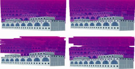
Figure 5.19 The top two images are examples of 1-variable orbital pictures, rendered using a version of IFS colouring. The condensation picture is in the foreground of each image. The bottom two images represent 2-variable orbital pictures. All four pictures are associated with the same superIFS, which consists of two affine IFSs on R2.

the sequence {Pσ1σ2···σk (P0)}∞k=1 provides a unique picture, much as in Theorem 3.5.3. We denote this picture by

Pσ (P0) = lim Pσ1σ2···σk (P0).

k→∞

We refer to Pσ (P0) as the 1-variable orbital picture associated with F(1), the condensation picture P0 and the string σ {1,2,...,M}.

Here is the crucial bit of algebra: for all P0 C(X), m {1, 2, . . . , M} and

σ {1,2,...,M} {1,2,...,M} we have

Pmσ (P0) = P0 Fm (Pσ (P0)).

This tells us that we may use the chaos game to approximate and sample the set of 1-variable orbital pictures {Pσ (P0) : σ {1,2,...,M}}. We define a random orbit

Pk (P0) according to

Pk+1(P0) = P0 Fσk (Pk (P0)) with P1(P0) = P0

for k = 1, 2, . . . , where σk is chosen equal to m with probability Pm , independently of all other choices.

The upper two images in Figure 5.19 provide two examples of 1-variable orbital pictures. The condensation picture P0 is represented by the pale-blue building in the foreground. I modified the colours of successive panels by IFS colouring to yield a stable picture on the ‘horizon’. To see more correctly the mathematical orbital pictures you should imagine that each building is the same colour as the

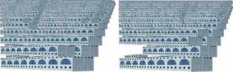
Figure 5.20 Two different 1-variable underneath pictures, generated using a superIFS and a condensation picture; the latter is represented by the building in the foreground. Many different sequences of underneath pictures may be obtained by random iteration. Such sequences of pictures may in practice display a ‘texture effect’ as illustrated here, near the horizon.

one in the foreground. The 1-variable IFS F(1) used here consists of two affine IFSs, which in turn consist of two transformations each. You should be able to deduce these transformations approximately by studying the two images. I was for a while quite mesmerized by the sequence of fantasy cities which appeared on my computer screen.

By now, you should be able to make a good guess at the definition of a 2-variable orbital picture. Examples of 2-variable orbital pictures are given in the bottom two panels of Figure 5.19 and also in Figure 5.26.

Collections of 1-variable underneath pictures

The superIFS in Equation (5.4.1) may be used to define a set of transformations

←−

F m : C(X) → C(X) by

for all P0 C(X) and for m = 1, 2, . . . , M. Then we define

for all σ {1,2,...,M}. We may generate corresponding random orbits of 1-variable underneath pictures {Pk (P0)}∞k=1with the aid of the chaos game, according to

for k = 1, 2, . . . , where, as elsewhere, σk is chosen as equal to m with probability Pm , independently of all other choices.

In computational examples these random orbits behave in a very similar manner to the sequences of underneath pictures discussed in Section 3.5. For example, Figure 5.20 illustrates the ‘texture effect’ in several 1-variable underneath pictures corresponding to the same superIFS.

414 Superfractals

Random orbits of 1-variable pictures

The superIFS

{X; F1, F2, . . . , FM ; P1, P2, . . . , PM }

may be used to define transformations Fm : C(X) → C(X) by

for all P0 C(X) and for m = 1, 2, . . . , M. Then we define

Fσ (P0) := Fσ1 ◦ Fσ2 ◦ · · · ◦ Fσ|σ | (P0)

for σ {1,2,...,M} to be a 1-variable picture. We may generate corresponding random orbits of 1-variable pictures {Pk (P0)}∞k=1 with the aid of the chaos game,

according to

Pk+1(P0) = Fσk (Pk (P0)) with P1(P0) = P0,

for k = 1, 2, . . . , where, as elsewhere, σk is chosen equal to m with probability Pm , independently of all other choices. Similarly defined random orbits of measures, starting from a measure μ0 P(X), approach elements of A and similarly defined random orbits of sets, starting from a set C0 H(X), approach elements of A(1), in each case in the manner already described. The random orbit of pictures {Pk (P0)}∞k=1, however, typically does not converge to a limiting superfractal of pictures, in the sense of asymptotically dancing around on some limiting object, for essentially the same reason that the deterministic sequence of pictures {F◦k (P0)}∞k=1 does not in general converge to a well-defined picture, as discussed in Section 4.8. In computational examples we find that random orbits of 1- variable pictures often display texture effects, as do the analogous random orbits of V -variable pictures. The restless pattern of purple dots on green 2-variable ‘ti-trees’ in Figure 5.24 illustrates this phenomenon.

Directed sets of 1-variable fractal sets

We can use the superIFS {X; F1, F2, . . . , FM } together with a shift-invariant closed subset of {1,2,...,M} to define the directed 1-variable IFS (F(1), ). The theory from Section 4.16 and onwards in Chapter 4 comes into play and may be interpreted in the present setting. The deterministic fractal set associated with (F(1), ) consists of a set of compact subsets of X.

To show that it is useful to think about directed 1-variable IFSs, we note the following. By choosing the structure of appropriately, say to have a recurrent or graph-directed form, it is possible to design algorithms, along the lines of the chaos game, which yield for example families of ‘1-variable’ overlapping ferns that generalize those illustrated in Figure 4.37. Also, it appears straightforward to provide conditions on the superIFS under which the boundaries of the elements of the attractor A(1) of the IFS F(1) are related to the deterministic fractal set associated

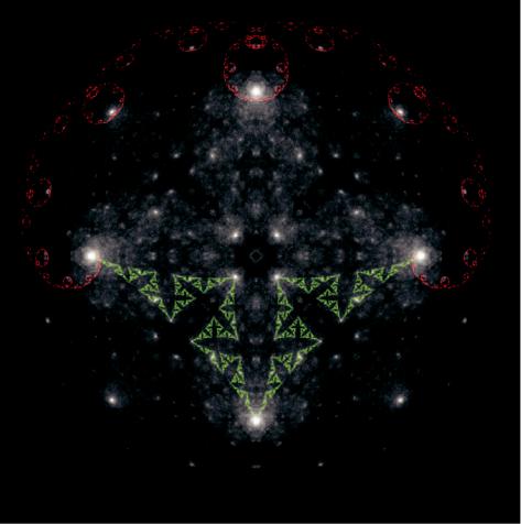
Figure 5.21 This illustrates symbolically the 2-variable superfractal associated with the computational experiment in Section 5.2. What you actually see is the superposition of many of the 2-variable sets, tethered curves, treated as measures. The bright points correspond to a high density of curves. The red and green curves represent the attractors of the two IFSs that generate the superfractal.

with a directed 1-variable IFS of the form (F(1), ), being defined appropriately. Such a result may be proved similarly to the proof of Theorem 4.16.6.

5.12V -variable IFSs

We begin by describing the transformations that are implicit in the computational experiment in Section 5.2, generalized to the case where we have V buffers in place of two buffers. So if you have trouble initially in seeing what the following formulas mean, take V = 2 and think about how you would write down one of the transformations between the ‘input screens’ and ‘output screens’ in Section 5.2. See Figure 5.21.

≤ λ · dHV (B1, B2, . . . , BV ), (C1, C2, . . . , CV ) .

It follows that F(V ) possesses a unique set attractor

A(V ) H H(X)V .

It must also possess a unique measure attractor

μ(V ) P H(X)V .

We refer to the set

A(V ) = B H(X) : B is a component of a point in A(V )

as the V -variable superfractal associated with F(V ) and we refer to its elements as V -variable fractal sets. Notice that A(1) = A(1) and that

A(1) A(2) A(3) · · · H(H(X)).

For V ≥ 2 the elements of A(V ) are not in general directly related to set attractors of compositions of the Fm . But, for example, if M ≥ 4 then A(2) contains such vectors of sets as (A12, A3412) and (A1, Aσ ), where Aσ A(1); A(V ) contains many other types of set, however.

The chaos game corresponding to the IFS F(V ) may be used to produce sequences of points, V -tuples of compact sets, in A(V ), asymptotically distributed according to the probability measure μ(V ).

where A(vV ) denotes the set comprising the vth components of the elements of A(V ). If the probabilities in F(V ) are given by Equation (5.12.2) then, starting from any initial V -tuple of nonempty compact subsets of X, the random distribution of the sets comprising the vth components of the first K vectors produced by the chaos game converges weakly to the marginal probability measure

Theorem 5.12.2 tells us that we can sample the superfractal A(V ) by means of the chaos game applied to the IFS F(V ). To do this we define sequences of vectors of nonempty compact subsets of X by

starting from any point (B11, B21, . . . , BV1 ) H(X)V . Here

ak = a A with probability pa

independently of all other choices, a is given by Equation (5.12.1) and pa is given by Equation (5.12.2). The sequence of measures

μ(KV ) = K −1 δB11 + δB12 + · · · + δB1K

belonging to the space P(H(X)) converges weakly as K → ∞, almost always, to the same probability measure in P(H(X)), namely the measure μ(V ) defined by Equation (5.12.3).

An example in which we use the chaos game to compute samples of a 2-variable superfractal is provided by the computational experiment in Section 5.2. In this case the superfractal is equivalent to a family of continuous paths tethered at two points, and the observed stationary state corresponds to the measure μ(2).

In Figure 5.22 we illustrate some 2-variable fractal sets associated with the superIFS used to produce Figure 5.7, discussed in Section 5.6. See Figure 5.23 for a close-up of one of these sets. The 2-variable fractal sets here have been rendered using a version of colour-stealing. When V ≥ 2 colour-stealing works somewhat differently from the case V = 1, because the chaos game does not preserve even a ‘local’ tops structure, as mentioned in Section 5.13 below.

The arrows in Figure 5.22 help to explain the 2-variability of these images. The two arrows attached to a set point to the parents of the set. Each set is a union of three or four transformations applied to one or other of its parents. Furthermore,

Figure 5.22 This illustrates successive pairs of 2-variable sets, in reverse order, produced by the chaos game. Each arrow points from a ‘child’ to one of its ‘parents’; the pair of arrows emanating from each set shows the result of applying the transformation T to the set, as explained in Section 5.18.

the parents are siblings, both having the same parents. And so on back through history. Thus, if you look closely at any set in the figure you can see either the parent or, when there are two parents, both parents. You can also see, as though homununculi within homunculi, all the grandparents and all the great-grandparents. There are at most two forebears in each generation. The arrows also illustrate the structure of a dynamical system belonging to the superfractal, which we discuss in more detail in Section 5.18.

During the chaos game, of course, we travel in the opposite direction, from parents to children. The images 1a and 1b were used to compute 2a and 2b, which were used to compute 3a and 3b, which were used to compute 4a and 4b, which were used to compute 5.