Ohrimenko+ / Barnsley. Superfractals

Figure 4.27 The tops dynamical system associated with the IFS F1 in Equations (4.9.1) and (4.14.2). The tops code space and its closure can be found, in quite a straightforward way, by thinking about the possible structures of orbits such as the one illustrated in the figure.

of F together with all strings that can be written in the form

11 · · · 122 · · · 2122 · · · 2122 · · · 212.

Code structures associated with dynamical systems of the form seen in Figure 4.27 have been extensively studied in the context of information theory and symbolic dynamics; see for example papers in the literature that cite [82]. The complexity and richness of this one very simple example suggests that endless wonders await those who explore simple nontrivial two-dimensional situations.

E x e r c i s e 4.14.2 Find the code space structure for the IFS, given in Table 4.2, which makes a Sierpinski triangle.

E x e r c i s e 4.14.3 Describe, roughly, the code space structure for the overlapping IFS in Table 4.4.

D e f i n i t i o n 4.14.4 Let F and G be two hyperbolic IFSs. We say that the code structures of F and G are homeomorphic if there is a homeomorphism

χ : F → G which respects the code structures, that is, which maps each set in the code structure of F onto a set in the code structure of G.

If F is a totally disconnected IFS and G is obtained from F by permuting the order of the functions in F then clearly the code space structures of F and G are homeomorphic. Other examples of homeomorphic code structures, involving overlapping IFSs, can also be exhibited. But for the most part it is convenient to think of χ as the identity map.

T h e o r e m 4.14.5 Let the code structures of two hyperbolic IFSs F and G be homeomorphic. Then their set attractors, AF and AG, are homeomorphic. That is, there exists a continuous one-to-one invertible transformation H : AF → AG such that

H ( AF ) = AG.

We remark that if the tops code spaces of two hyperbolic IFSs F and G are the same then their set attractors are related by the one-to-one invertible transformation H : AF → AG defined by

H = τG−1 ◦ τF .

But, in general, this transformation is not continuous because of the possible discontinuity of τF .

the attractors be denoted by AF XF and AG XG respectively. Let the code

space functions be denoted by φF : {1,2,...,NF } → AF and φG : {1,2,...,NG} → AG respectively and let the tops code spaces be denoted by F and G respectively.

Let the tops functions be denoted by τF : AF → F and τG : AG → G respectively. Now let the homeomorphism between code structures, asserted in the theorem, be denoted by

χ : F → G.

Then we claim that the transformation H : AF → AG defined by

H = φG ◦ χ ◦ τF

provides the desired homeomorphism between the attractors.

It is useful to notice at this stage that H is a one-to-one invertible transformation between the two attractors. You can readily verify that its inverse is given by

H −1 = φF ◦ χ −1 ◦ τG = τF−1 ◦ χ −1 ◦ τG.

We need to show that it is continuous. This follows from a subtle observation and a theorem in elementary topology.

The subtle observation, by Mendelson [70], p. 194, is this. If F : X → Y is a continuous mapping of a compact space X onto a Hausdorff space Y then the topology of Y is the same as the identification topology induced by F.

This tells us that the identification topology on AF , which is induced by the

code space mapping φF : {1,2,...,NF } → AF restricted to F , is the same as the natural topology on AF , as a subset of the metric space XF .

The theorem we apply is Proposition 7.4 of [70], p. 195. Let X, Y and Z be topological spaces. Let F : X → Y be onto and let Y have the identification topology induced by F. Then the function H : Y → Z is continuous iff the composition G := H ◦ F : X → Z is continuous.

We choose F : X → Y to be φF : F → AF and H : Y → Z to be

H = φG ◦ χ ◦ τF : AF → AG.

Then F : X → Y is onto and, as we pointed out above, the topology of Y = AF is the same as the identification topology and also the natural topology. Now look at the function

G := H ◦ F = φG ◦ χ ◦ τF ◦ φF : F → AG.

If σ F then (τF ◦ φF )(σ ) belongs to the same set in the code space structure of F as σ . Since χ respects the code space structure, both χ (σ ) and (χ ◦ τF ◦ φF )(σ ) belong to the same set in the code space structure of G. It follows that

(φG ◦ χ ◦ τF ◦ φF )(σ ) = (φG ◦ χ )(σ ) for all σ F .

But φG ◦ χ : F → AG is the composition of two continuous maps, and so it is continuous. It follows that G is continuous and therefore that H is continuous. Similarly, its inverse is continuous. Hence H is a homeomorphism.

E x e r c i s e 4.14.6 Prove Mendelson’s subtle observation, above. The key is to note that if f : X → Y is continuous, where X and Y are topological spaces, and if C is a compact subset of X then f (C) is a compact subset of Y.

E x e r c i s e 4.14.7 Prove Proposition 7.4 of [70], quoted above.

The idea that the tops code space is roughly, but not precisely, the same as the code structure of an IFS is a convenient aide memoire, but remember to take the closure.

C o r o l l a r y 4.14.8 Let A denote the set of all set attractors of all hyperbolic IFSs. Then

A, B A are homeomorphic A and B possess the same code space structure.

Figure 4.28 To find an IFS whose attractor is a Mobius¨ strip, first colour the Mobius¨ strip pink and white, as in (i), to help illustrate the transformations. Next, flatten the strip to make a rectangle whose top looks like (ii) and whose bottom looks like (iii). Then make four shrunken copies (iv) of the rectangle and join them to form a new rectangle (v). Then twist and join the composite figure (v) to form a second Mobius¨ strip (vi). Note that the code structure of the resulting IFS cannot be the same as that of any IFS whose attractor lies in R2.

P r o o f Theorem 4.14.5 yields . To prove , suppose that A, B A are homeomorphic. Then there exists a hyperbolic IFS F = { A; f1, f2, . . . , fN }, with set attractor AF = A, and a metric d such that ( A, d) is a compact metric space. There also exists a homeomorphism H : A → B with H ( A) = B. Then it is readily verified that the IFS

One consequence of the corollary is that there can exist no code structure, for a set such as a circle, a figure eight or a Sierpinski triangle, that is also a code structure for a set that is contained in R; for otherwise the circle, figure-eight or Sierpinski triangle would be homeomorphic to a subset of R, which clearly is not true. In Figure 4.28 we suggest how you might find a code structure for a Mobius¨ strip. The resulting code structure could not also belong to an IFS on R2.

364 Hyperbolic IFSs, attractors and fractal tops

T h e o r e m 4.14.9 (Fractal homeomorphism theorem) With the same set-up

and notation as above, let the homeomorphism χ : F → G have the property χ ( F ) = G. Then

τG = χ ◦ τF ◦ H −1,

where H : AF → AG is the continuous one-to-one invertible transformation from AF onto AG given in Theorem 4.14.5. Moreover the tops dynamical systems TF : AF → AF and TG : AG → AG are topologically conjugate according to

TG = H ◦ TF ◦ H −1.

P r o o f This follows immediately from the proof of Theorem 4.14.5. The stated identities turn on the facts that (τF ◦ φF )(σ ) = σ for all σ F and that we have restricted the homeomorphism χ : F → G so that it maps from F onto G.

When dynamical systems are topologically conjugate they may share many properties, as discussed in Section 3.5.

When the drawing IFS FD and the colouring IFS FC have the same code structure, the relationship between the stolen picture PD and PC is precisely

H (PD ) = PC |AC .

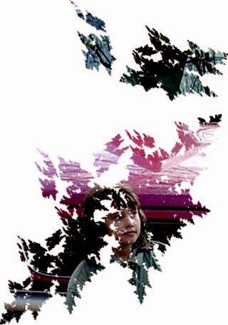
That is, PD is a continuous invertible transformation of PC restricted to the domain of the colouring IFS. We will discuss this relationship further in Section 4.15. A consequence, which has never failed to surprise colleagues to whom I have demonstrated it, in video applications, is that if FD = FC then PD = PC . This is illustrated in Figure 4.29.

Here, briefly, let me suppose that a hyperbolic IFS F in R3 is a model of botanical meristem: in the development of the set attractor of F, which I think of as a geometrical model for an entity in plant physiology, such as phloem or the veins within a leaf, I see the expression of the code structure of F in the topology of the intricate tangle of proteins that comprises the botanical entity. The locations in space of the amino acids in the proteins, both in sequences along strands and adjacently at different points along the same or different strands, may then be considered as a physical manifestation of the identification topology induced by φF : F → AF . Is it possible, in a realistic practical way, to make a mathematical model for the veins of a leaf using a simple IFS and so provide a reasonable connection between the physical development, via DNA and meristem, and the decoding of the IFS?

Figure 4.29 In this example of colour-stealing, the same IFS has been used both to draw and to coloursteal. The attractor of the IFS is the domain of this picture.

4.15Fractal transformations

In this section we study more closely the relationship, implicit in colour-stealing, between some pairs of set attractors. In so doing we alert you, the sharp-eyed reader, to some areas of application of fractal tops and colour-stealing. For simplicity of presentation we restrict the discussion to the case where there is a single underlying compact metric space X. Let F = {X; f1, f2, . . . , fN } and G = {X; g1, g2, . . . , gN } denote hyperbolic IFSs on X. Let AF and AG denote their respective set attractors, F and G denote their tops code spaces, τF : AF → F and τG : AG → G denote their tops functions and φF : → AF and φG : → AG denote their respective code space functions.

D e f i n i t i o n 4.15.1 The transformation FG : AF → AG defined by

FG = φG ◦ τF

is called a fractal transformation from AF into AG.

Fractal transformations underlie colour-stealing. To see this, suppose that we choose FD = F and FC = G. Also, suppose without loss of generality that DPC = AG. Then the relationship between the stolen picture PF := PD and the picture PG := PC from which the colours were stolen is

There are three quite distinct situations which can occur. Each corresponds to a different kind of relationship between PF and PG. We treat these situations separately.

(i) F = G. In this case, in general the tops transformation FG is neither one-to-one nor onto. But from Theorem 4.11.5 we know that it is ‘nearly’ continuous, at least when fn is a homeomorphism between X and fn (X) for each n {1, 2, . . . , N }. Thus, in this case FG is continuous on AinsideF ; its discontinuities are restricted to certain pre-images, possibly a countable dense set of lines, of the boundary of AF . This partially explains the look-and-feel of some stolen pictures, as follows. A set of fractal boundaries, transformed copies of the boundary of AF , provide what we refer to as ‘line-art’ on AF , and FG is continuous at all other points of AF ; hence, as x varies over AinsideF , FG(x) varies continuously over the domain of the picture PG while the colour at FG(x) is given to the point x. Insofar as the colours PG(y) depend continuously on y, the colours painted on AF will vary continuously away from the line-art.

It is important, though, to notice that in general, in this case, we cannot think of PF as being the result of applying a transformation to PG as described in Chapter 2, because FG is not invertible.

A simple example of colour-stealing when the tops transformation is not one- to-one is illustrated by the top right image in Figure 4.30. Here the line-art consists of portions of boundaries of many rectangles. You will see that bits of the rocks are missing. It is as though parts of the stolen picture have been put underneath other parts. The picture PC from which colours were stolen is shown at the top left. The IFSs F = F1 and G are illustrated in Figure 4.31. The code structure of G is essentially that of the unit square written in quadtree representation, but the code structure of F1 omits many addresses in the code structure of G because its tops dynamical system behaves in much the same way as that of the IFS in Equation (4.14.1) above, in both the x- and y- directions. Many potential addresses are simply wiped out by the overlapping region. In Figure 4.31, at upper right, we

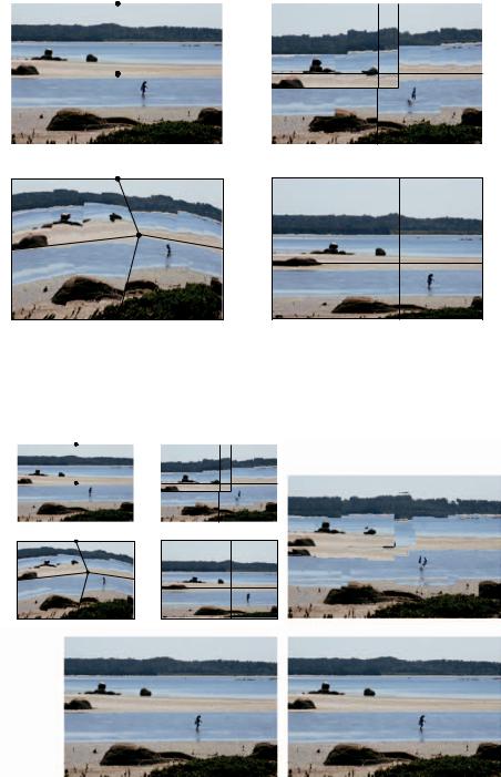
368 Hyperbolic IFSs, attractors and fractal tops

show the result of reversing the colour-stealing process, with PC = PF , FC = F1 and FD = G; clearly we do not get back to the original picture!

(ii) F = G, but the code structures of F and G are different. In this case the fractal transformation FG maps AF one-to-one onto AG, but in general it is not continuous. Its inverse is −FG1 = GF = φF ◦ τG. In particular, we have

PG = GF (PF ).

In this case, we do get back to the original picture from the stolen one when we reverse the colour-stealing process; specifically,

PF = FG(PG).

In practice we achieve this inversion by swapping the colouring and drawing IFSs and using the previously stolen picture as the one from which to steal the colours. This technique has immediate application to image encryption and to copyright protection. It is also provides a novel method for changing the distribution of information in a picture, by first transforming to a stolen picture, then filtering and then transforming back. This is relevant to image-compression applications.

An example of case (ii) is shown in the bottom left panel of Figure 4.30. Here you can see that FG is not continuous; it has discontinuities associated with the line-art, which consists of segments of conic sections. The picture PC is shown at the top left, and the IFSs F = F2 and G are illustrated in Figure 4.31. The latter figure also illustrates the result (see the bottom left image) of applying the inverse of the transformation to the transformed image; although not exactly the same as the original, it is accurate to within computational errors. These errors are due mainly to discretization.

How do we know that F2 = G? By considering the tops dynamical systems of F2 and G. It is straightforward to prove that σ is the code of an orbit of TF2 iff it is an orbit of TG. How do we know that the code structures of F2 and G are different, in this example? One can prove this by comparing the sets of addresses of points on the line ab in Figure 4.31, provided by the IFS G, with those of points on the line a b , provided by the IFS F2. These structures are quite different, because the former are provided by superimposing two standard binary codings of a line segment, whereas the latter correspond to the superposition of two mismatched ‘projective’ binary codings of a line segment.

(iii) The code structures of F and G are the same. In this case FG is precisely the homeomorphism H : AF → AG provided in Theorems 4.14.5 and 4.14.9 when χ = 1. An example is shown in the bottom right panel of Figure 4.30. Here you can see that FG is continuous. The IFSs F = F3 and G are illustrated in

Figure 4.32 Example of a fractal transformation. These two pictures are homeomorphic, by the fractal homeomorphism theorem.

Figure 4.33 Before and after a fractal transformation. Which is before?

Figure 4.31, which also shows the result (see the bottom right image) of applying the inverse of the homeomorphism to the transformed image.

The code structures of F3 and G are the same because both collages are made of affine transformations. The problem of mismatching binary codings, mentioned at the end of point (ii), is resolved; in this case they match.

Two other examples of homeomorphic fractal transformations are illustrated in Figures 4.32 and 4.33. These use similar IFSs to the pair used in (iii) above.