Narayanan V.K., Armstrong D.J. - Causal Mapping for Research in Information Technology (2005)(en)

130 Srivastava, Buche and Roberts

a significant positive impact on ‘Job Satisfaction’ as seen from Figure 6. As the belief in opportunity to use new skills increases, the belief in job satisfaction increases. We find an 8.5% increase in job satisfaction over the range from 0 – 1.0 for belief in opportunity to use new skills. This impact is linear, unlike the previous case.

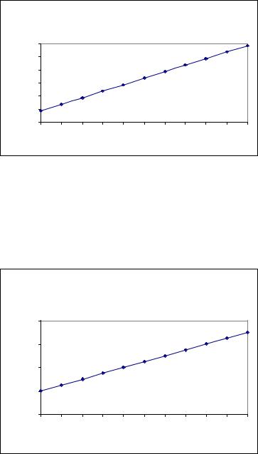
The third variable analyzed is ‘Feedback from Supervisors/Co-workers’. As shown in Figure 7, the results demonstrate a substantial positive impact of feedback on the job satisfaction. In particular, job satisfaction increases about 19% as we progress from the lower to higher levels of perceived feedback. It is obvious that feedback is a powerful variable in predicting job satisfaction.

Next, we conduct a sensitivity analysis with the independent variable, ‘Challenging Work’. ‘Job Satisfaction’ was extremely sensitive to increases in the perceived level of challenging work. From no belief that the job is challenging to the higher range of belief, 1.0, the model indicates that the belief in job satisfaction moves from 0.388 to 0.838; a 129% increase as seen in Figure 8. These results indicate that challenging work is the most powerful variable in the model in the prediction of job satisfaction.

Finally, a sensitivity analysis was conducted on ‘Autonomy of Work’. The results indicate that ‘Autonomy of Work’ has a significant impact on the dependent variable, ‘Job Satisfaction’. Job satisfaction was found to be very sensitive to autonomy. As the perceived autonomy increases from 0 to 1.0, job satisfaction improves from 60% to 85%, an increase of 41.6%. These results are presented in Figure 9.

These sensitivity analyses have shown the impact on job satisfaction from a broad range of variables and their corresponding beliefs. However, we do want to point out that the

Figure 7. Belief in job satisfaction versus belief in feedback from supervisors and coworkers*

Impact of Belief in Feedback from Supervisors and Co-Workers on Belief in Job Satisfaction

Belief in Feedback from Supervisors and Co-Workers

*The following input m-values in Figure 4 were used for the graph: mE1(yesRR)=0, mE1(noRR)=0,

mE2.1(yesJT)=0.27, mE2.1(noJT)=0.73, mE2.2(yesJT)=0, mE2.2(noJT)=0, mE3(yesST)=0, mE3(noST)=0, mE4(yesGS)=0, mE4(noGS)=0, mE5(yesUS)=0.81, mE5(noUS)=0, mE6(yesFS) varied from 0 - 1, mE6(noFS)=0, mE7(yesCW)=0.81, mE7(noCW)=0, mE8(yesAW)=0.77, mE8(noAW)=0.23.

Copyright © 2005, Idea Group Inc. Copying or distributing in print or electronic forms without written permission of Idea Group Inc. is prohibited.

Belief Function Approach to Evidential Reasoning in Causal Maps 131

Figure 8. Belief in job satisfaction versus belief in challenging work*

Figure 9. Belief in job satisfaction versus belief in autonomy of work*

Copyright © 2005, Idea Group Inc. Copying or distributing in print or electronic forms without written permission of Idea Group Inc. is prohibited.

132 Srivastava, Buche and Roberts

interrelationships among the intermediate variables and the relative weights assigned to ‘Opportunity to use New Skills’, ‘Feedback from Supervisors and Co-Workers, ‘Challenging Work’, and ‘Autonomy of Work’, have direct impact on the results for the dependent variable, ‘Job Satisfaction’.

In summary, the above analysis provides an example of how an evidential reasoning approach under Dempster-Shafer theory of belief functions can be used to determine the impact on a given construct or constructs of other constructs in a revealed causal map. It should be noted that a revealed causal map of a decision problem is only a static model while an evidential diagram of a revealed causal map provides a dynamic model for analyzing the behaviors of various constructs under different conditions.

Conclusions and Future Directions for Research

In this chapter we have demonstrated the use of evidential reasoning approach under Dempster-Shafer (D-S) theory of belief functions to analyze revealed causal maps. As an example, we used a simplified causal map obtained through a Revealed Causal Mapping (RCM) technique where the participants were from information technology (IT) organizations who provided the concepts to describe the target phenomenon of ‘Job Satisfaction’. They also identified the associations between the concepts. After creating the causal map of the problem being investigated, we developed an evidential diagram. This diagram consists of the variables or constructs of the causal map, interconnected to the other variables with some relationships. These relationships were defined by the decision maker based on experience. Various items of evidence were identified that pertained to different variables. Estimates of the beliefs in terms of m-values in support of, or negation of, the variables were made for each item of evidence using survey questions (Buche, 2003, particularly Appendix C). These m-values were then propagated through the evidential network to obtain the overall belief of ‘Job Satisfaction’.

To illustrate the usefulness of the evidential reasoning approach under Dempster-Shafer theory of belief functions, we performed various sensitivity analyses to determine the impact of different variables on ‘Job Satisfaction’. This technique enables researchers to predict the level of job satisfaction when given evidence for the other variables in the model. As further validation for our findings, our results are directly in line with previous literature on job satisfaction for workers in general. IT personnel are very similar to other professions and vocations. An evidential diagram similar to the one discussed here would be useful in predicting whether a specific work environment would be more or less satisfactory to an employee before joining the job.

In this chapter we have explained the steps necessary to convert revealed causal maps into evidential diagrams. The analysis of the transformed diagram is useful in forming predictions about human behavior. This technique incorporates the existence of uncertainty in the level of belief associated with the evidence. Therefore, the researcher is able

Copyright © 2005, Idea Group Inc. Copying or distributing in print or electronic forms without written permission of Idea Group Inc. is prohibited.

Belief Function Approach to Evidential Reasoning in Causal Maps 133

to include in the diagram personal intuition and confidence based on direct experience. Another advantage of the evidential reasoning approach over a revealed causal map is that the former provides a dynamic model of a decision problem while the later provides only a static model. As a limitation, the evidential reasoning approach may become quite complex especially when variables or constructs in the diagram are highly integrated. For ease of instruction, the example discussed herein was fairly simplistic, with primarily linear associations.

References

Ang, S., & Slaughter, S.A. (2001). Work outcomes and job design for contract versus permanent information systems professionals on software development teams.

MIS Quarterly, 25, 321-350.

Axelrod, R. (1976). Structure of decisions: The cognitive maps of political elites. Princeton, NJ: Princeton University Press.

Bougon, M.G., Weick, K., & Binkhorst, D. (1977). Cognition in organizations: An analysis of the Utrecht Jazz Orchestra. Administrative Science Quarterly, 22, 606-639.

Bovee, M, Srivastava, R. P., & Mak, B. (2003, January). A conceptual framework and belief-function approach to assessing overall information quality. International Journal of Intelligent Systems, 18(1), 51-74.

Buche, M.W. (2003). IT professional work identity: Constructs and outcomes. Unpublished dissertation, University of Kansas, Lawrence, KS.

Carley, K. (1997). Extracting team mental models through textural analysis. Journal of Organizational Behavior, 18, 533-558.

Curley, S. P., & Golden, J.I. (1994). Using belief functions to represent degrees of belief.

Organization Behavior and Human Decision Processes, 271-303.

Darais, K.M., Nelson, K.M., Rice, S.C., & Buche, M.W. (2003). Identifying the enablers and barriers of IT personnel transition. In C. Shayo & M. Igbaria (Eds.), Strategies for managing IS/IT personnel (pp. 92-112). Hershey, PA: Idea Group.

Gupta, Y.P., Guimaraes, T., & Raghunathan, T.S. (1992). Attitudes and intentions of information center personnel. Information & Management, 22, 151-160.

Hackman, J.R., & Oldham, G. (1976). Motivation through the design of work: Test of a theory. Organizational Behavior and Human Performance, 16, 250-279.

Harrison, K., Srivastava, R.P., & Plumlee, R.D. (2002). Auditors’ Evaluations of Uncertain Audit Evidence: Belief Functions versus Probabilities. In R. P. Srivastava & T. Mock (Eds.), Belief functions in business decisions, (pp. 161-183). Heidelberg: Springer-Verlag.

Huff, A.S. (1990). Mapping strategic thought. Chichester, UK: Wiley.

Copyright © 2005, Idea Group Inc. Copying or distributing in print or electronic forms without written permission of Idea Group Inc. is prohibited.

134 Srivastava, Buche and Roberts

Igbaria, M., & Guimaraes, R. (1993). Antecedents and consequences of job satisfaction among information center employees. Journal of Management Information Systems, 9, 145-174.

Markoczy, L., & Goldberg, J. (1995). A method for eliciting and comparing causal maps.

Journal of Management, 21, 305-333.

Nadkarni, S., & Shenoy, P.P. (2001). A Bayesian Network approach to making inferences in causal maps. European Journal of Operational Research, 128, 479-498.

Narayanan, V.K., & Fahey, L. (1990). Evolution of revealed causal maps during decline: A case study of Admiral. In A. Huff (Ed.). Mapping strategic thought (pp. 109-133). London: John Wiley & Sons.

Nelson, K.M. (2000). IT personnel transition and organization transition strategy. National Science Foundation Grant.

Nelson, K.M., Nadkarni, S., Narayanan, V.K., & Ghods, M. (2000). Understanding software operations support expertise: A causal mapping approach. MIS Quarterly, 24, 475-507.

Pearl, J. (1990). Bayesian and belief-functions formalism for evidential reasoning: a conceptual analysis. In Readings in uncertain reasoning (pp. 540-574). San Mateo, CA: Morgan Kaufmann.

Radding, A. (1997). Rock-solid incentives. Network World, 14, 31-34.

Saffiotti, A., & Umkehrer, E. (1991). Pulcinella: A general tool for propagating uncertainty in valuation networks. Proceedings of the Seventh National Conference on Artificial Intelligence (pp. 323-331), University of California, Los Angeles.

Shafer, G. (1976). A mathematical theory of evidence. Princeton University Press.

Shafer, G., Shenoy, P.P., & Srivastava, R.P. (1988, May). Auditor’s Assistant: A knowledge engineering tool for audit decisions. Proceedings of the 1988 Touche Ross/University of Kansas Symposium on Auditing Problems (pp. 61-79).

Shafer, G., & Srivastava, R.P. (1990). The Bayesian and belief-function formalisms: A general perspective for auditing. Auditing: A Journal of Practice and Theory, (Supplement), 110-148.

Shenoy, P.P. (1991). Valuation-based system for discrete optimization. In P.P. Bonissone, M. Henrion, L. N. Kanal, and J. Lemmer (Eds.), Uncertainty in artificial intelligence, (Vol. 6, pp. 385-400). Amsterdam: North-Holland.,

Shenoy, P.P., & Shafer, G. (1990). Axioms for probability and belief-function propagation. In Uncertainty in artificial intelligence. Elsevier Science Publishers.

Smets, P. (1998). The transferable belief model for quantified belief representation. In P. Smets (Ed.), Quantified representation for uncertainty and imprecision, (Vol. 1). Kluwer Academic Publishers.

Smets, P. (1990a, May). The combination of evidence in the transferable belief model.

IEEE Transactions on Pattern Analysis and Machine Intelligence, 12, 5.

Copyright © 2005, Idea Group Inc. Copying or distributing in print or electronic forms without written permission of Idea Group Inc. is prohibited.

Belief Function Approach to Evidential Reasoning in Causal Maps 135

Smets, P. (1990b). Constructing the pignistic probability function in a context of uncertainty. In M. Henrion, R.D. Shachter, L.N. Kanal & J F. Lemmer (Eds.),

Uncertainty in artificial intelligence 5. North-Holland: Elsevier Science Publishers B.V.

Srivastava, R.P. (1995, March). The belief-function approach to aggregating audit evidence. International Journal of Intelligent Systems, 10(3), 329-356.

Srivastava, R.P. (1993, Fall). Belief functions and audit decisions. Auditors Report, 17(1), 8-12.

Srivastava, R.P., & Datta, D. (2002). Belief-function approach to evidential reasoning for acquisition and merger decisions. In R. P. Srivastava & T. Mock (Eds.), Belief functions in business decisions (pp. 220-248). Heidelberg: Springer-Verlag.

Srivastava, R.P., & Liu, L. (2003). Applications of belief functions in business decisions: A review. Information Systems Frontiers (forthcoming).

Srivastava, R.P., & Lu, H. (2002, October). Structural analysis of audit evidence using belief functions. Fuzzy Sets and Systems, 131(1), 107-120.

Srivastava, R.P., & Mock, T.J. (2002). Belief functions in business decisions. Heidelberg: Springer-Verlag.

Srivastava, R.P., & Mock, T.J. (2000, Winter). Evidential reasoning for Webtrust assurance services. Journal of Management Information Systems, 10(3), 11-32.

Strat, T.M. (1984). Continuous Belief functions for evidential reasoning. Proceedings of the National Conference on Artificial Intelligence, Austin, Texas (pp. 308-313).

Thatcher, J.B., Stepina, L.P., & Boyle, R.J. (2002-2003). Turnover of information technology workers: Examining empirically the influence of attitudes, job characteristics, and external markets. Journal of Management Information Systems, 19, 231-261.

Wrightson, M.T. (1976). Coding rules. In R. Axelrod (Ed.), Structure of decisions: The cognitive maps of political elites (pp. 291-332). Princeton, NJ: Princeton University Press.

Zarley, D. Y. T., & Shafer, G. (1988). Evidential Reasoning using DELIEF. Proceedings of the National Conference of Artificial Intelligence.

Endnotes

1See the following references for more discussion on belief functions and their applications: Bovee et al. (2003), Srivastava (1993), Srivastava and Datta (2002), Srivastava and Liu (2003), and Srivastava and Mock (2000).

2For three independent items of evidence, Dempster’s rules can be written as:

Copyright © 2005, Idea Group Inc. Copying or distributing in print or electronic forms without written permission of Idea Group Inc. is prohibited.

136 Srivastava, Buche and Roberts

One can easily generalize the above formula for n independent items of evidence (see Shafer, 1976, for details).

3The argument of m-function represents the state for which the value is assigned and the subscript describes the evidence from which the value is derived. For

example, mX(x) = 0.6 represents 0.6 level of support for ‘x’ from an item of evidence pertaining to the variable X.

4Propagation is the process by which m-values on a variable or a set of variables are moved (mapped) to another variable or a set of variables. For example, m-values from variable X in Figure 1 can be propagated to the relational variable ‘AND’ that consist of three variables, X, Y, and Z.

5Vacuous extension is the process through which m-values on a smaller frame are extended to a larger frame. For example, m(x) when vacuously extended to the joint space of X and Y, i.e., the frame {xy, x~y, ~xy, ~x~y}, yields m(x) = m({xy, x~y}).

6Marginalization of m-values is opposite to the vacuous extension. This process is similar to marginalization in probability theory; it involves eliminating all the unwanted variables by summing the m-values over the unwanted variables. For example, assume that we have the following m-values on the joint space of X and

Y, ΘX,Y ={xy,x~y,~xy,~x~y}:m({xy})=0.1,m({xy,x~y})=0.6,andm({xy,x~y,~xy, ~x~y}) = 0.3. The marginalized m-values onto the space of X variable are: m({x}) = 0.1 + 0.6 = 0.7, and m({x, ~x}) = 0.3. Similarly, the marginalized m-values onto the Y space are: m({y}) = 0.1, m({y, ~y}) = 0.9.

7Through this example we are illustrating the details of the propagation process of beliefs or m-values through a tree of variables as this is what is needed in our model of IT job satisfaction obtained through the RCM process. A discussion on the details of the propagation of beliefs through a network of variables is beyond the scope of this chapter. Interested readers should see Srivastava (1995) and Shenoy and Shafer (1990) for this kind of propagation.

8A Markov tree is characterized by a set of nodes N and a set of edges E where each edge is a two-element subset of N such that (Srivastava, 1995; see also, Shenoy, 1991):

• (N,E) is a tree.

•If N and N’ are two distinct nodes in N, and {N, N’} is an edge, i.e., {N,N'} E , then Ν∩N’≠ .

•If N and N’ are distinct nodes of N, and X is a variable in both N and N’, then X is in every node on the path from N to N’.

Copyright © 2005, Idea Group Inc. Copying or distributing in print or electronic forms without written permission of Idea Group Inc. is prohibited.

Belief Function Approach to Evidential Reasoning in Causal Maps 137

9As described in Section IV, in order to propagate m-values from ‘RR’ to ‘JT’ through the relationship R1, one needs to vacuously extend the m-values from the space

of ‘RR’, {yesRR, noRR}, to the space of R1, which is the joint space of ‘RR’ and ‘JT’, i.e., {(yesRR, yesJT), (yesRR, noJT), (noRR, yesJT), (noRR, noJT)}, combine the m-values at R1, and then marginalize to the space of ‘JT’, {yesJT, noJT}.

10This semi-structured interview guide was also part of NSF grant proposal and Transition Study research project (Nelson, 2000; Buche, 2003).

Appendix A: Concept Dictionary with Examples

Copyright © 2005, Idea Group Inc. Copying or distributing in print or electronic forms without written permission of Idea Group Inc. is prohibited.

138 Srivastava, Buche and Roberts

Appendix B: Interview Protocol10

1.What motivates you to come to work here every day?

2.What is the best thing about your current work environment?

3.What is the worst thing about your current work environment?

4.What is the most important thing you contribute to this organization?

5.What could you contribute to your organization that you currently are unable to contribute?

6.What barriers keep you from making this contribution?

7.Where do you realistically see yourself professionally in five years?

8.Where would you ideally like to see yourself professionally in five years?

9.What barriers might keep you from your ideal situation?

10.How much do you like change?

11.How much do you think the IT field, in general, is changing?

12.How much do you think the IT field at your company is changing?

13.How do you feel about this level of change?

14.How is your organization supporting you in personally making these changes?

15.What barriers do you see in making these changes?

16.What is your primary, one year professional goal?

17.How can your organization help you achieve you goals?

18.In summary, how do you see yourself fitting into the organization’s “big picture”?

19.Would you like to add any further comments or observations?

Appendix C: Propagation Illustration in

Figure 1

In this appendix we describe in detail the three steps involved in the propagation of m- values from variables X and Y in Figure 1 to variable Z.

Step 1: Propagation of m-values from X and Y to ‘AND’ node:

In order to propagate m-values from variable X, a smaller node with one variable and the frame ΘX={x,~x}, to the ‘AND’ node, a larger node consisting of three variable X, Y, and

Copyright © 2005, Idea Group Inc. Copying or distributing in print or electronic forms without written permission of Idea Group Inc. is prohibited.

Belief Function Approach to Evidential Reasoning in Causal Maps 139

Z with the frame ΘAND= {xyz, x~y~z, ~xy~z, ~x~y~z}, we vacuously extend the m-values at X to the space {xyz, x~y~z, ~xy~z, ~x~y~z} defined by the ‘AND’ node. This process yields the following non-zero m-values from X to the ‘AND’ node:

mAND←X({xyz, x~y~z}) = mX(x) = 0.6, mAND←X({~xy~z, ~x~y~z}) = mX(~x) = 0.2,

mAND←X({xyz, x~y~z, ~xy~z, ~x~y~z}) = mX({x, ~x}) = 0.2.

Similarly, we obtain the following non-zero m-values at the ‘AND’ node when the m- values from Y are propagated to the ‘AND’ node:

mAND←Y({xyz, ~xy~z}) = mY(y) = 0.7

mAND←Y({xyz, x~y~z, ~xy~z, ~x~y~z}) = mY({y,~y}) = 0.3

Step 2: Combine m-values from X and Y with the m-values at ‘AND’

We have the following set of m-values at the ‘AND’ node; one from X, one from Y, and one at the ‘AND’ node defining the relationship.

m-values from X:

mAND←X({xyz, x~y~z}) = 0.6, mAND←X({~xy~z, ~x~y~z}) = 0.2, and mAND←X({xyz, x~y~z, ~xy~z, ~x~y~z}) = 0.2.

m-values from Y:

mAND←Y({xyz, ~xy~z}) = 0.7,

mAND←Y({xyz, x~y~z, ~xy~z, ~x~y~z}) = 0.3.

m-values at the ‘AND’ node:

mAND({xyz, x~y~z, ~xy~z, ~x~y~z}) = 1.0.

After we combine the above m-values using Dempster’s rule, we obtain the following m- values:

Copyright © 2005, Idea Group Inc. Copying or distributing in print or electronic forms without written permission of Idea Group Inc. is prohibited.