Narayanan V.K., Armstrong D.J. - Causal Mapping for Research in Information Technology (2005)(en)

120 Srivastava, Buche and Roberts

network which then provides the aggregated m-values at each cluster of variables in the network. One can then analyze how one variable impacts another variable by making changes in the input m-values in the network.

Since the evidential diagram in our case is a simple tree, it is pretty straight forward to propagate m-values through such a tree as described Appendix C. In order to analyze the model in Figure 4, we develop a spreadsheet program that combines different m-values at each variable and then propagates them through the tree to the desired variable. This process is elaborated in Section VI.

Illustration of Evidential Reasoning:

Causal Map of IT Job Satisfaction

Job satisfaction of information technology (IT) workers has been the focus of several information systems studies (e.g., Igbaria & Guimaraes, 1993; Gupta et al., 1992; Thatcher et al., 2003). Organizations want to retain their best IT workers as long as they possess the skills necessary to accomplish the job. However, there is growing concern that many long term IT employees no longer fit the needs of their employers.

The general consensus from the research is that job satisfaction is negatively related to turnover intention (e.g., Thatcher et al., 2003). In other words, workers who are highly satisfied with their jobs are less likely to contemplate seeking other employment and many unsatisfied workers enter the job market. In the current environment of radical role changes (Darais et al., 2003) and selectivity in hiring, IT workers within firms are experiencing anxiety and frustration, wondering what skills they will need to remain marketable in the future. The current trend with offshoring many IT jobs has exacerbated this problem for many workers. IT workers with traditionally secure positions are not immune to the pressures of this dynamic job environment.

In the present study, the IT Professional Job Satisfaction Model was developed based on 83 discovery interviews with IT workers in various job positions including systems analysts, programmers, technical specialists, and systems project managers. Table 3 shows the demographics for the interview sample.

These workers were from eight different corporations in a variety of industries (e.g., banking and insurance, manufacturing, education, state and local government). They voluntarily discussed their opinions on a number of job-related issues, generally focusing on their feelings of uncertainty regarding their personal contributions and job security (see the Interview Protocol in Appendix B). Interviews were generally 30 – 45 minutes in length and tape recorded, with the consent of the participant. Then, the interviews were transcribed and the causal statements were highlighted and analyzed according to the RCM technique described in Section II of this chapter. The causal map (Figure 3) was created based on the concepts represented in the transcripts.

In analyzing the data, one clear finding is that most of the IT personnel interviewed had difficulty describing how they fit within the corporate structure. They acknowledged that

Copyright © 2005, Idea Group Inc. Copying or distributing in print or electronic forms without written permission of Idea Group Inc. is prohibited.

Belief Function Approach to Evidential Reasoning in Causal Maps 121

Table 3. Interview sample demographics

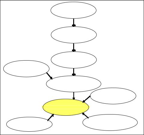
their contributions were important, but they felt they were personally expendable. Several persons similarly stated, “I’m just a cog in the wheel.” As many researchers and practitioners have noted (e.g., Darais et al., 2003), in order to survive in the IT field, workers must continue to retrain and learn new skills. Therefore, acknowledgement of the need to change is depicted as the first node in the IT Professional Job Satisfaction Model (see Figure 3, Item 1). The interviewees indicated that skills stagnation often threatened job security. This realistic fear of job loss (Figure 3, Item 2) is a powerful motivator in pursuing necessary training.

IT workers in the interviews discussed the importance of seeking out training opportunities (Figure 3, Item 3), whether offered by the corporation as in-house training, enrollment in formal college courses, or on-line, computer-aided learning. These courses might entail attaining certification credentials, college credit, or practical experience. According to a majority of interviewees, if training is available at the place of work, and offered during work hours, employees are more likely to take advantage of the instruction. In contrast, off-hours training, to be completed outside of work on one’s personal time, was less attractive to these employees. However, there is no guarantee that participation in training courses produces adequate knowledge for accomplishing new tasks.

Beyond merely gaining new knowledge and skills (Figure 3, Item 4), interviewees stressed that they must also be able to practice and apply the new skills in a meaningful way (Figure 3, Item 5). In other words, they believe that their training must be utilized on work projects in order for the new skills to become part of workers’ permanent skill sets. Unfortunately, technical skills are often lost if they are not used soon after the course is completed (Radding, 1997).

Some of the relevant elements of job satisfaction (Figure 3, Item 9) that emerged from this study were perceived feedback from supervisors and co-workers (Figure 3, Item 6),

Copyright © 2005, Idea Group Inc. Copying or distributing in print or electronic forms without written permission of Idea Group Inc. is prohibited.

122 Srivastava, Buche and Roberts

participation in challenging projects (Figure 3, Item 7), and autonomy within the work setting (Figure 3, Item 8). Many IT projects involve teams working together to accomplish defined objectives. Direct feedback obtained from supervisors and co-workers (Figure 3, Item 6) increases job satisfaction because there is less ambiguity about perceived performance. For instance, the interviewees stated that they like to receive continuous feedback in order to determine whether they have adequately satisfied the user requirements and specifications during systems development.

Next, challenging projects (Figure 3, Item 7) provide intrinsic motivation for IT workers. Interviewees remarked that they were anxious to tackle difficult problems for the basic joy of simply discovering new solutions. But, beyond the initial pleasure of design development is the pride of successful implementation and user adoption of their creative solutions. These accomplishments instill job satisfaction at a deep level for IT problemsolvers.

Figure 3. Information technology professional job satisfaction model

Copyright © 2005, Idea Group Inc. Copying or distributing in print or electronic forms without written permission of Idea Group Inc. is prohibited.

Belief Function Approach to Evidential Reasoning in Causal Maps 123

Finally, the level of autonomy (Figure 3, Item 8) positively affects job satisfaction because most IT employees prefer freedom and independence in determining relevant job-related decisions (Ang & Slaughter, 2001; Hackman & Oldham, 1976). According to the interviewees, they derive positive affect from exercising autonomy in project completion, resulting in increased job satisfaction.

Table 4 shows evidence used to support the construct measures. For this study, evidence was obtained from survey data. The survey was developed as an extension of a study in which the RCM technique was used to develop a model of work identity for IT professionals (Buche, 2003). Other possible examples of evidence would be additional interviews, observation, evaluation of documentation, and reviewing physical artifacts. Some of the elements could be gathered from supervisors and secondary sources, triangulating the evidence to analyze the model and to predict job satisfaction of IT professionals.

Table 4. Variables, symbols and respective sources of evidence

Copyright © 2005, Idea Group Inc. Copying or distributing in print or electronic forms without written permission of Idea Group Inc. is prohibited.

124 Srivastava, Buche and Roberts

Conversion of Revealed Causal Map into Evidential Diagram and Belief Propagation

In this section we first discuss how a revealed causal map can be converted to a belief function evidential diagram and then discuss how beliefs can be propagated through this evidential diagram. Our example is displayed in Figure 3.

Conversion of Revealed Causal Map into Evidential Diagram

The conversion process of revealed causal map into evidential diagram can be described in the following five steps:

1.Identify the main variables (i.e., constructs) in the revealed causal map.

2.Determine the possible values of these variables (such as, ‘true/false’, or ‘high/ medium/low’).

3.Determine the relationships among the variables (see the details below).

4.Connect the variables through the corresponding relationships.

5.Identify potential items of evidence pertaining to the variables in the diagram and connect these items of evidence to the relevant variables.

The above approach yields the desired evidential diagram for belief-function analysis. In Steps 1 and 2, we have identified nine variables (i.e., constructs; see Figure 3) and their corresponding categorical values (Table 4).

Step 3 (determining the relationships among various variables) is a somewhat difficult process. Expert judgments about these relationships must be rendered. For example, the relationship R1 defining the relationship between ‘Role Recognition (RR)’ and ‘Job Security (JT)’ was extremely difficult to model. In this case, the survey data provided only information on whether the subjects recognize their changing role on the job and did not specify any details on how this knowledge might influence ‘Job Security’. For IT personnel, ‘Role Recognition’ might mean that ‘yes’ there is ‘Job Security’, but it also may mean that there is no ‘Job Security’. Thus, lacking any other information, we assume, for the present discussion, that when ‘Role Recognition’ is yes, ‘Job Security’ is 50% ‘yes’, and 50% ‘no’. However, when there is no knowledge about ‘Role Recognition’, there is no knowledge about ‘Job Security’. Such a relationship can be expressed in terms of m-values as given below.

Copyright © 2005, Idea Group Inc. Copying or distributing in print or electronic forms without written permission of Idea Group Inc. is prohibited.

Belief Function Approach to Evidential Reasoning in Causal Maps 125

m-values for R1:

mR1({(yes RR, yes JT), (no RR, yes JT), (no RR, no JT)}) = 0.5, mR1({(yes RR, no JT), (no RR, yes JT), (no RR, no JT)}) = 0.5.

The above relationship propagates9 50% of mE1(yes RR), the belief on ‘Role Recognition’ being ‘yes’ from evidence E1 (Figure 4), to ‘yesJT’ 50% of mE1(yesRR) to ‘noJT’, and 100%

of mE1(noRR) and mE1({yesRR, noRR}) to ({yesJT, noJT}), as described in the assumed relationship. In other words, the m-values propagated from variable ‘Role Recognition

(RR)’ to variable ‘Job security (JT)’ are given as:

mJT←RR(yesJT) = 0.5mE1(yesRR), mJT¬RR(noJT) = 0.5mE1(yesRR), and mJT←RR({yesJT, noJT}) = mE1(noRR) + mE1({yesRR, yesRR})

For the relationship R2 we assume the following. On average, a person with the knowledge that there is no job security will sign up for job training with 90% belief and a person with the knowledge that there is no problem with the job security will not sign up for job training with 90% belief. This relationship can be modeled in the following way:

m-values for R2:

mR2({(yes JT, no ST), (no JT, yes ST)}) = 0.9, and

mR2({(yes JT, yes ST), (yes JT, no ST), (no JT, yes ST), (no JT, no ST)}) = 0.1.

Similar to endnote 9, one can easily show the following m-values to be the result of m- values propagated from variable ‘Job Security (JT)’ to variable ‘Sign up for Job Training (ST)’ through the relationship R2:

mST←JT(yesST) = 0.9mJT(noJT), mST¬JT(noST) = 0.9mJT(yesJT), and mST←JT({yesST, noST}) = 0.1 + 0.9mJT({yesRR, yesRR}).

We assumed the following m-values for R3 (see Table 4 for the definitions of the symbols):

m-values for R3:

mR3({(yes ST, yesUS), (no ST, no US)}) = 0.75, and

mR3({(yes ST, yes US), (yes ST, no US), (no ST, yes US), (no ST, no US)}) = 0.25.

Copyright © 2005, Idea Group Inc. Copying or distributing in print or electronic forms without written permission of Idea Group Inc. is prohibited.

126 Srivastava, Buche and Roberts

The relationship previously discussed implies that if variable ‘ST’ is ‘yes’, i.e., a person sings up for training, then variable ‘US’ will be ‘yes’, i.e., the person will have the opportunity to use the new skill with 0.75 belief, and the remaining 0.25 belief is assigned to ignorance. Similarly, the relationship implies that if ‘ST’ is ‘no’ then ‘US’ is ‘no’ with belief 0.75, i.e., if one does not sign up for job training then he/she will not have the use of new skill with belief 0.75. The remaining 0.25 belief represents ignorance.

For the relationship R4, we assume the following m-values:

m-values for R4:

mR4({(yesGS, yesUS), (noGS, noUS)}) = 1.0.

This relationship implies that if ‘GS’ is ‘yes’ then ‘US’ is ‘yes’ with 1.0 belief. Also, if ‘GS’ is ‘no’ then ‘US’ is ‘no’ with 1.0 belief. In other words, if one has the opportunity to gain new skills on the job then there is 1.0 belief that there is opportunity to use the new skills. Similarly, if there is no opportunity to gain new skills on the job then there is no opportunity to use the new skills.

The relationship R5 relates variables ‘US’, ‘FS’, ‘AW’, and ‘CW’ to the variable ‘Job Satisfaction (JS)’. We have assumed the following relative weights, 0.125, 0.125, 0.25, and 0.5, respectively, for ‘US’, ‘FS’, ‘AW’, and ‘CW’ when propagating information (m- values) to the variable ‘JS’.

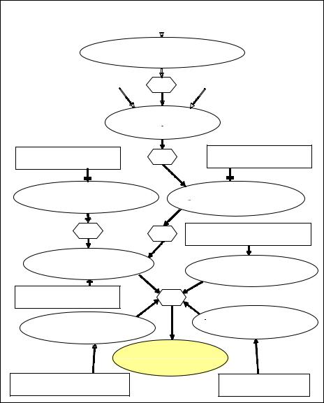
Step 4 simply represents a diagram with all the variables interconnected through the assumed relationships (see Figure 4). In Step 5, we identify various items of evidence pertaining to different variables and connect them to the corresponding variables. Table 4 provides a list of evidence pertaining to the nine variables in Figure 4. Once these items of evidence are connected to the corresponding variables, we develop the evidential diagram shown in Figure 4 for the analysis.

Propagation of Beliefs through Evidential Diagram

In order to propagate information in terms of m-values from all the variables to the variable of interest, say, ‘Job Satisfaction (JS)’ in Figure 4, we need to follow the following steps. First, gather all the information (m-values) at ‘Role Recognition (RR)’, propagate that information (m-values) to variable ‘Job Security (JT)’ through the relationship R1 by first vacuously extending to the space of R1, combining it with the m-values at R1 using Dempster’s rule, and then marginalizing the resulting m-values to the space of ‘JT’. Combine this information (m-values) with the m-values at ‘JT’ obtained from evidence E2.1 and E2.2, again using Dempster’s rule. Next step is to propagate the resulting m- values at ‘JT’ through R2 to the variable ‘Sign up for Training to Gain New Skills (ST)’. This is achieved again by vacuously extending the total m-values at ‘JT’ to the space of R2, combining them with the m-values at R2 using Dempster’s rule, and then marginalizing them to the space of variable ‘ST’. Combine this information (m-values) with the m-values obtained from evidence E3 for ‘ST’. The resulting m-values are then propagated to the

Copyright © 2005, Idea Group Inc. Copying or distributing in print or electronic forms without written permission of Idea Group Inc. is prohibited.

Belief Function Approach to Evidential Reasoning in Causal Maps 127

variable ‘Opportunity to use New Skills (US)’. Combine these m-values with the m-values obtained from the variable ‘Opportunity to Gain New Skills on the Job (GS)’ and the m- values from evidence E5 for ‘US’.

In the final step, we need to propagate all the m-values from the four variables, ‘US’, ‘FS’, ‘AW’, and ‘CW’ through the relationship R5 to the variable ‘Job Satisfaction (JS)’ by vacuously extending the respective m-values to the space of R5, combine these m-values with the m-values defining R5 and then marginalize them to the space of ‘Job Satisfaction’. The marginalized m-values on ‘Job Satisfaction (JS)’ can be written as:

mJS(yesJS) = 0.125mUS(yesUS) + 0.125mFS(yesFS) + 0.25mAW(yesAW) + 0.5mCW(yesCW). mJS(noJS) = 0.125mUS(noUS) + 0.125mFS(noFS) + 0.25mAW(noAW) + 0.5mCW(noCW).

mJS({yesJS, noJS}) = 1 - mJS(yesJS) - mJS(noJS).

These m-values provide the impact of all the variables in the evidential diagram in Figure 4.

Given that the evidential diagram in Figure 4 is a tree, the propagation of m-values from various variables to the variable of interest, ‘Job Satisfaction’ is much easier than propagation in a network of variables. We programmed the logic of vacuous extension, marginalization, and Dempster’s rule of combination in a spreadsheet program in MS Excel, which then was used to perform various analyses as discussed in the next section.

Decision Analysis of Causal Map Using

Belief Functions

In this section, we discuss how one can analyze the impact of one variable on the other variables in the network given in Figure 4. Such an analysis allows the decision maker to isolate an independent variable while holding the rest of the variables in the model constant. In this example, the overall belief in job satisfaction is 0.803 given the inputs from the Survey Results and industry data. The above value implies that based on the subjects responses, on average, employees are satisfied with their jobs in the environment surveyed with 0.803 level of belief. In order to investigate the impact of a number of variables on the level of job satisfaction, we use a range of possible responses (0 to 1.0) for the variables while keeping the inputs from other items of evidence fixed at values obtained from the survey as given in the respective figures.

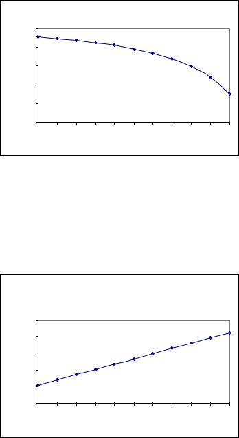
First, we investigate the impact of ‘Job Security’ on ‘Job Satisfaction’. We vary the input belief from evidence E2.2 for the negation of ‘Job Security’ from 0 to 1.0, keeping the rest of inputs fixed. As seen in Figure 5, the impact of ‘No Job Security’ is pretty severe. As the belief in no job security increases the belief in job satisfaction decreases with increasing rate. In other words, if an employee sees strong evidence in support of ‘no job security’ then he/she will have very low job satisfaction.

The second sensitivity analysis is conducted on the impact of having an opportunity to use new skills on the job. This analysis reveals that the opportunity to use new skills has

Copyright © 2005, Idea Group Inc. Copying or distributing in print or electronic forms without written permission of Idea Group Inc. is prohibited.

128 Srivastava, Buche and Roberts

Figure 4. Evidential diagram* of the causal map in Figure 3

*The oval shaped boxes represent variables and the rectangular boxes represent items of evidence. The numbers in a rectangular box represent the level of support for and against the variable it is connected to. These numbers were determined from the Survey Results except for E2.1 which

was determined from the industry data.

Copyright © 2005, Idea Group Inc. Copying or distributing in print or electronic forms without written permission of Idea Group Inc. is prohibited.

Belief Function Approach to Evidential Reasoning in Causal Maps 129

Figure 5. Belief in job satisfaction versus belief in no job security*

*The following input m-values in Figure 4 were used for the graph: mE1(yesRR)=0, mE1(noRR)=0,

mE2.1(yesJT)=0.27, mE2.1(noJT)=0.73, mE2.2(yesJT)=0, mE2.2(noJT)=0, mE3(yesST)=0, mE3(noST)=0, mE4(yesGS)=0, mE4(noGS)=0, mE5(yesUS) varied from 0 - 1, mE5(noUS)=0, mE6(yesFS)=0.66, mE6(noFS)=0.34, mE7(yesCW)=0.81, mE7(noCW)=0, mE8(yesAW)=0.77, mE8(noAW)=0.23.

Figure 6. Belief in job satisfaction versus belief in opportunity to use new skills*

Impact of Belief in Opportunity to use New Skills on Belief in Job

Satisfaction

Belief in Opportunity to use New Skills

*The following input m-values in Figure 4 were used for the graph: mE1(yesRR)=0, mE1(noRR)=0,

mE2.1(yesJT)=0.27, mE2.1(noJT)=0.73, mE2.2(yesJT)=0, mE2.2(noJT)=0, mE3(yesST)=0, mE3(noST)=0, mE4(yesGS)=0, mE4(noGS)=0, mE5(yesUS) varied from 0 - 1, mE5(noUS)=0, mE6(yesFS)=0.66, mE6(noFS)=0.34, mE7(yesCW)=0.81, mE7(noCW)=0, mE8(yesAW)=0.77, mE8(noAW)=0.23.

Copyright © 2005, Idea Group Inc. Copying or distributing in print or electronic forms without written permission of Idea Group Inc. is prohibited.