Narayanan V.K., Armstrong D.J. - Causal Mapping for Research in Information Technology (2005)(en)

110 Srivastava, Buche and Roberts

and prediction. An example is provided to demonstrate these steps. This chapter also provides the basics of Dempster-Shafer theory of belief functions and a step-by-step description of the propagation process of beliefs in tree-like evidential diagrams.

Introduction

The main purpose of this chapter is to demonstrate the use of evidential reasoning approach under Dempster-Shafer (D-S) theory of belief functions (Shafer, 1976; see also, Srivastava & Datta, 2002; and Srivastava & Mock, 2000, 2002) to analyze revealed causal maps. The Revealed Causal Mapping (RCM) technique is used to represent the model of a mental map and to determine the constructs or variables of the model and their interrelationships from the data. RCM focuses on the cause/effect linkages disclosed by individuals intimately familiar with a phenomenon under investigation. The researcher deliberately avoids determining the variables and their associations a priori, allowing both to emerge during the discourse or from the textual analysis (Narayanan & Fahey, 1990). In contrast, other forms of causal mapping begin with a framework of variables based on theory, and the associations are provided by the participants in the study (cf. Bougon, et al., 1977).

While RCM helps determine the significant variables in the model and their associations, it does not provide a way to integrate uncertainties involved in the variables or to use the model to predict future behavior. The evidential reasoning approach provides a technique where one can take the RCM model, convert it into an evidential diagram, and then use it to predict how a variable of interest would behave under various scenarios. An evidential diagram is a model showing interrelationships among various variables in a decision problem along with relevant items of evidence pertaining to those variables that can be used to evaluate the impact on a given variable of all other variables in the diagram. In other words, RCM is a good technique to identify the significant constructs (i.e., variables) and their interrelationships relevant to a model, whereas evidential approach is good for making if-then analyses once the model is established.

There are two steps required in order to achieve our objective. One is to convert the RCM model to an evidential diagram with the variables taken from the RCM model and items of evidence identified for the variables from the problem domain. The second step is to deal with uncertainties associated with evidence. In general, uncertainties are inherent in RCM model variables. For example, in our case of IT professionals’ job satisfaction, the variable “Feedback from Supervisors/Co-Workers” partly determines whether an individual will have a “high” or “low” level of satisfaction. However, the level of job satisfaction will depend on the level of confidence we have in our measure of the variable. The Feedback from Supervisors/Co-Workers may be evaluated through several relevant items of evidence such as interviews or surveys. In general, such items of evidence provide less than 100% assurance in support of, or negation of, the pertinent variable. The uncertainties associated with these variables are better modeled under DempsterShafer theory of belief functions than probabilities as empirically shown by Harrison, Srivastava and Plumlee (2002) in auditing and by Curley and Golden (1994) in psychology.

Copyright © 2005, Idea Group Inc. Copying or distributing in print or electronic forms without written permission of Idea Group Inc. is prohibited.

Belief Function Approach to Evidential Reasoning in Causal Maps 111

We use belief functions to represent uncertainties associated with the model variables and use evidential reasoning approach to determine the impact of a given variable on another in the model. This combination of techniques adds the strength of prediction to the usefulness of descriptive modeling when studying behavioral phenomena. Evidential reasoning under Dempster-Shafer theory of belief functions thereby extends the impact of revealed causal mapping.

The chapter is divided into eight sections. Section II provides a brief description of the Revealed Causal Mapping (RCM) technique. Section III discusses the basic concepts of belief functions, and provides an illustration of Dempster’s rule of combination of independent items of evidence. Section IV describes the evidential reasoning approach under belief functions. Section V describes a causal map developed through interviews and surveys of IT employees on their job satisfaction. Section VI shows the process of converting a RCM map to an evidential diagram under belief functions. Section VII presents the results of the analysis, and Section VIII provides conclusions and directions for future research.

Revealed Causal Mapping Technique

Revealed causal mapping is a form of content analysis that attempts to discern the mental models of individuals based on their verbal or text-based communications (Carley, 1997; Darais et al., 2003; Narayanan & Fahey, 1990; Nelson et al., 2000). The general structure of the causal map can reveal a wealth of information about cognitive associations, explaining idiosyncratic behaviors and reasoning.

The actual steps used to develop the IT Job Satisfaction revealed causal map in the present paper are outlined in Table 1. The research constructs were not determined a priori, but were derived from the assertions in the data. The sequence of steps directly develops the structure of the model from the data sample.

First, a key consideration in using RCM is the determination of source data (Narayanan & Fahey, 1990). Since this study assessed the job satisfaction of IT professionals, it was logical to gather data from IT workers in a variety of industries. Interviews were conducted with employees of IT departments, and responses were analyzed to produce the model presented later in the chapter.

Second, the researchers identified causal statements from the original transcripts or documents. The third step in the procedure is to combine concepts based on coding rules

Table 1. Steps for revealed causal mapping technique

Copyright © 2005, Idea Group Inc. Copying or distributing in print or electronic forms without written permission of Idea Group Inc. is prohibited.

112 Srivastava, Buche and Roberts

(Axelrod, 1976; Wrightson, 1976), producing a concept dictionary (see Appendix A). Synonyms are grouped to enable interpretation and comparison of the resultant causal maps. Care must be taken to ensure that synonyms are true to the original conveyance of the participant. For example, two interviewees might use different words that hold identical or very similar meanings such as “computer application” and “computer program.” In mapping these terms, the links are not identical until the concepts are coded by the researcher. It is preferable for investigators to err on the side of too many concepts, rather than inadvertently combine terms inappropriately for the sake of parsimony.

Next, the maps of the individual participants were aggregated by combining the linkages between the relevant concepts. The result of this step is a representative causal map for the sample of participants (Markoczy & Goldberg, 1995).

RCM produces dependent maps, meaning that the links between nodes indicate the presence of an association explicitly revealed in the data (Nadkarni & Shenoy, 2001). The absence of a line does not imply independence between the nodes, however. It simply means that a particular link was not stated by the participants. This characteristic of RCM demonstrates the close relationship of the graphical result (map) to the data set. Therefore, it is vital that the sample be representative of the population of interest. The following section introduces belief functions and the importance of evidential reasoning in managerial decision making.

Dempster-Shafer Theory of Belief

Functions

Dempster-Shafer (D-S) theory of belief functions, which is also known as the belieffunction framework, is a broader framework than probability theory (Shafer and Srivastava, 1990). Actually, Bayesian framework is a special case of belief-function framework. The basic difference between the belief-function framework and probability theory or Bayesian framework is in the assignment of uncertainties to a mutually exclusive and collectively exhaustive set of elements, say Θ,with elements {a1, a2, a3,...an}. This set of elements, Θ = {a1, a2, a3,...an}, is known as a frame of discernment in belief-function framework. In probability theory, probabilities are assigned to individual elements, i.e., to the singletons, and they all add to one. For example, for the frame, Θ ={a1, a2, a3, … an}, with n mutually exclusive and collectively exhaustive set of elements, ai’s, with i = 1, 2, 3, … n, one assigns a probability measure to each element, 1.0 ≥ P(ai) ≥ 0, such that

n

∑P(ai ) = 1.

i=1

Under belief functions, however, the probablity mass is distributed over the super set of the elements Θ instead of just the singletons. Shafer (1976) calls this probability mass distribution the basic probability assignment function, whereas Smets calls it belief masses (Smets 1998, 1990a, 1990b). We will use Shafer’s terminology of probability mass distribution over the superset of Θ.

Copyright © 2005, Idea Group Inc. Copying or distributing in print or electronic forms without written permission of Idea Group Inc. is prohibited.

Belief Function Approach to Evidential Reasoning in Causal Maps 113

Basic Probability Assignment Function (m-Values)

In the present context, the basic probability assignment function represents the strength of evidence. For example, suppose that we have received feedback from a survey of the IT employees of a company about whether their work is challenging or not. On average, the employees believe that their work is challenging but they do not say this with certainty; they put a high level of comfort, say 0.85 (on a scale 0 – 1.0), that their work is challenging. But, they do not say that their work is not challenging. This response can be represented through the basic probability assignment function, m-values1, on the frame, {‘yesCW’, ‘noCW’}, of the variable ‘Challenging Work (CW)’ as: m(yesCW) = 0.85, m(noCW) = 0, and m({yesCW, noCW}) = 0.15. These values imply that the evidence suggests that the work is challenging to a degree 0.85, it is not challenging to a degree zero (there is no evidence in support of the negation), and it is undecided to a degree 0.15.

Mathematically, the basic probability assignment function represents the distribution of probability masses over the superset of the frame, Θ. In other words, probability masses are assigned to all the singletons, all subsets of two elements, three elements, and so on, to the entire frame. Traditionally, these probability masses are represented in

terms of m-values and the sum of all these m-values equals one, i.e., ∑ m(B) = 1 , where

BΘ

B represents a subset of elements of frame Θ. The m-value for the empty set is zero, i.e., m( ) = 0.

In addition to the basic probability assignment function, i.e., m-values, we have one other function, Belief function, represented by Bel(.), that is of interest in the present discussion. As defined below, Bel(A), determines the degree to which we believe, based on the evidence, that A is true. This function is discussed further below.

Belief Functions

The function, Bel(B), defines the belief in B, a subset of elements of frame Θ, that is true, and is equal to m (B) plus the sum of all the m-values for the set of elements contained

the definition. Based on the Survey Results, we have 0.85 level of belief that the employees have challenging work, zero belief that the employees do not have challenging work. This evidence can be mapped in the following belief functions by using the above definition:

Bel(yesCW) = m(yesCW) = 0.85, Bel(noCW) = m(noCW) = 0.0,

Bel({yesCW, noCW}) = m(yesCW) + m(noCW) + m({yesCW, noCW}) = 0.85 + 0.0 + 0.15 = 1.0.

Copyright © 2005, Idea Group Inc. Copying or distributing in print or electronic forms without written permission of Idea Group Inc. is prohibited.

114 Srivastava, Buche and Roberts

The belief values discussed previously imply that we have direct evidence from surveying the employees that the work is challenging to a degree 0.85, no belief that the work is not challenging, and the belief that the work is either challenging or not challenging is 1.0. Note that in our example there is no state or element contained in ‘yesCW’ or ‘noCW’. Thus, m-values and Bel(.) for these elements are the same.

Dempster’s Rule of Combination

Dempster’s rule of combination is similar to Bayes’ rule in probability theory. It is used to combine various independent items of evidence pertaining to a variable or a frame of discernment. As mentioned earlier, the strength of evidence is expressed in terms of m- values. Thus, if we have two independent items of evidence pertaining to a given variable, i.e., we have two sets of m-values for the same variable then the combined m-values are obtained by using Dempster’s rule. For a simple case2 of two items of evidence pertaining to a frame Θ. Dempter's rule of combination is expressed as:

m(B) = K-1. ∑ m1(Bi )m2 (Bj),

i,j

Bi∩Bj=B

where m(B) represents the strength of the combined evidence and m1 and m2 are the two sets of m-values associated with the two independent items of evidence. K is the renormalization constant given by:

K = 1 - ∑ m1(Bi )m2 (Bj).

i,j

Bi∩Bj=

The second term in K represents the conflict between the two items of evidence. When K = 0, i.e., when the two items of evidence totally conflict with each other, these two items of evidence are not combinable.

A simple interpretation of Dempster’s rule is that the combined m-value for a set of elements B is equal to the sum of the product of the two sets of m-values (from each item of evidence), m1(B1) and m2(B2), such that the intersection of B1 and B2 is equal to B and renormalize the m-values to add to one by eliminating the conflicts.

Let us consider an example to illustrate Dempster’s rule. Consider that we have the following sets of m-values from two independent items of evidence pertaining to a variable, say A, with two values, ‘a’, and ‘~a’, representing respectively, that A is true and is not true:

Copyright © 2005, Idea Group Inc. Copying or distributing in print or electronic forms without written permission of Idea Group Inc. is prohibited.

Belief Function Approach to Evidential Reasoning in Causal Maps 115

m1(a) = 0.4, m1(~a) = 0.1, m1({a, ~a}) = 0.5, m2(a) = 0.6, m2(~a) = 0.2, m2({a, ~a}) = 0.2.

As mentioned earlier, the general formula of Dempster’s rule yields the combines m-value for an element or a set of elements of the frame of discernment by multiplying the two sets of m-values such that the intersection of their respective arguments is equal to the element or set of elements desired in the combined m-value, and by eliminating the conflicts and renormalizing the resulting m-values such that the resulting m-values add to one. This reasoning yields the following expressions as a result of Dempster’s rule for binary variables:

m(a) = K-1[m1(a)m2(a) + m1(a)m2({a,~a}) + m1({a,~a})m2(a)],

m(~a) = K-1[m1(~a)m2(~a) + m1(~a)m2({a,~ a}) + m1({a,~ a})m2(~a)], m({a,~ a}) = K-1m1({a,~ a})m2({a,~ a}),

and

K = 1 – [m1(a)m2(~a) + m1(~a)m2(a)].

As we can see above, m(a) is the result of the multiplication of the two sets of m-values such that the intersection of their arguments is equal to ‘a’ and the renormalization constant, K, is equal to one minus the conflict terms. Similarly m(~a) and m({a,~a}) are the results of multiplying two sets of m-values such that the intersection of their arguments is equal to ‘~a’ and ({a,~a}), respectively.

Substituting the values for the two m-values, we obtain:

K = 1 – [0.4x0.2 + 0.1x0.6] = 0.86,

m(a) = [0.4x0.6 + 0.4x0.2 + 0.5x0.6]/0.86 = 0.72093, m(~a) = [0.1x0.2 + 0.1x0.2 + 0.5x0.2]/0.86 = 0.16279, m({a,~a}) = 0.5x0.2/0.86 = 0.11628.

Thus, the total beliefs after combining both items of evidence are given by:

Bel(a) = m(a) = 0.72093, Bel(~a) = m(~a) = 0.16279, and

Bel({a,~a}) = m(a) + m(~a) + m({a,~a}) = 0.72093 + 0.16279 + 0.11628 = 1.0.

The above values of beliefs in ‘a’ and ‘~a’ represent the combined beliefs from two items of evidence. Belief that ‘a’ is true from the first item of evidence is 0.4; from the second item of evidence it is 0.6, whereas the combined belief that ‘a’ is true based on the two

Copyright © 2005, Idea Group Inc. Copying or distributing in print or electronic forms without written permission of Idea Group Inc. is prohibited.

116 Srivastava, Buche and Roberts

items of evidence is 0.72093; a stronger belief as a result of the combination. The combined belief would have been much stronger if we did not have the conflict.

Evidential Reasoning Approach

Strat (1984) and Pearl (1990) have used the term “evidential reasoning” for decision making under uncertainty. Under this approach one needs to develop an evidential diagram (as shown in Figure 4 in the next section; see also Srivastava & Mock (2000) for other examples) containing all the variables involved in the decision problem with their interrelationships and the items of evidence pertaining to those variables. Once the evidential diagram is completed, the decision maker can determine the impact of a given variable on all other variables in the diagram by combining the knowledge about the variables. In other words, under the evidential reasoning approach, if we have knowledge about one or more variables in the evidential diagram, then we can make predictions about the other variables in the diagram given that we know how these variables are interrelated. Usually, the knowledge about the states of these variables is only partial, i.e., there is uncertainty associated with what we know about these variables. As mentioned earlier, we use Dempster-Shafer theory of belief functions to model these uncertainties.

In the present case, variables in the evidential diagram represent the “constructs” of the model obtained through the Revealed Causal Mapping (RCM) process, and the interrelationships represent how one variable or a multiple of variables influence a given variable. Such relationships among the variables can be defined either in terms of categorical relationships such as, ‘AND’, and ‘OR’, or in terms of uncertain relationships, such as a combination of ‘AND’ and ‘OR’, or some other relationships as discussed in the next section.

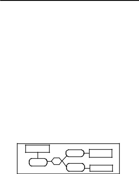
In order to illustrate the evidential reasoning approach, let us first construct an evidential diagram using a simple hypothetical decision problem involving three variables, X, Y, and Z (see Figure 1). Let us assume for simplicity that these variables are binary, i.e., each

Figure 1: Example of an evidential nework*

*Rounded boxes represent variables (constructs), hexagonal box represents a relationship, and rectangular boxes represent items of evidence pertinent to the variables they are connected

Copyright © 2005, Idea Group Inc. Copying or distributing in print or electronic forms without written permission of Idea Group Inc. is prohibited.

Belief Function Approach to Evidential Reasoning in Causal Maps 117

variable has two values: either the variable is true (x, y, and z) or false (~x, ~y, and ~z). Also, let us assume that variable Z is related to X and Y through the ‘AND’ relationship. This relationship implies that Z is true (z) if and only if X is true (x) and Y is true (y), but it is false (~z) when either X is true (x) and Y is false (~y), or X is false (~x) and Y is true (y), or both X and Y are false (~x, ~y). Now we draw a diagram consisting of the three variables, X, Y, and Z, represented by rounded boxes and connect them with a relational node represented by the hexagonal box. Further, connect each variable with the corresponding items of evidence represented by rectangular boxes. Figure 1 depicts the evidential diagram for the above case.

As mentioned earlier, an evidential reasoning approach helps us infer about one variable given what we know about the other variables in the evidential diagram. For example, in Figure 1, we can predict about the state of Z given what we know about the states of X and Y, and the relationship among them. Under the belief-function framework, this knowledge is expressed in terms of m-values. For example, knowledge about X and Y, based on the corresponding evidence, can be expressed in terms of m-values3, mX at X, and mY at Y, as: mX(x) = 0.6, mX(~x) = 0.2, mX({x,~x}) = 0.2, and mY(y) = 0.7, mY(~y) = 0, mY({y,~y}) = 0.3. The first set of m-values suggests that the evidence relevant to X provides 0.6 level of support that X is true, i.e., mX(x) = 0.6, 0.2 level of support that X is not true, i.e., mX(~x) = 0.2, and 0.2 level of support undecided, i.e., mX({x,~x}) = 0.2. One can provide a similar interpretation of the m-values for Y. The ‘AND’ relationship between X and Y, and Z can be expressed in terms of the following m-values: m({xyz, x~y~z, ~xy~z, ~x~y~z}) = 1.0. This relationship implies that z is true if and only if x is true and y is true, and it is false when either x is true and ~y is true, ~x is true and y is true, or ~x and ~y are true.

Based on the knowledge about X and Y above and the relationship of Z with X and Y, we can now make inferences about Z. This process consists of three steps which are described in Appendix C in detail. Basically, Step 1 involves propagating4 beliefs or m-

values from X and Y variables to the relational node ‘AND’ through vacuous5 extension. This process yields two sets of m-values at ‘AND’, one from X and the other from Y:

Table 2: List of symbols related to m-values used in the propagation process in Figure 1

Copyright © 2005, Idea Group Inc. Copying or distributing in print or electronic forms without written permission of Idea Group Inc. is prohibited.

118 Srivastava, Buche and Roberts

mAND←xand mAND←y (See Table 2 for definitions of symbols). Also, we already have one set of m-values, mAND, at the relational node ‘AND’. Step 2 involves combining the three sets of m-values at the ‘AND’ node using Dempster’s rule. Step 3 involves propagating the resulting m-values from the ‘AND’ node to variable Z by marginalization6. This

process yields mz←AND.These m-values are then combined with the m-values at Z, mZ, obtained from the evidence pertaining to Z. The resultant m-values will provide the belief

values whether Z is true or not true. As mentioned earlier, the details of the propagation process7 are discussed in Appendix C through a numerical example.

Modeling Uncertain Relationships among Variables

Srivastava and Lu (2002) have discussed a general approach to modeling various relationships under belief functions. We will use their approach to model the assumed relationships among various variables in Figure 4. As given earlier, the ‘AND’ relationship among X, Y and Z, under belief functions can be expressed in terms of the following m-value:

mAND({xyz, x~y~z, ~xy~z, ~x~y~z}) = 1.0.

The argument of m-value above determines the possible states of the joint space defining the ‘AND’ relationship. Similarly, the ‘OR’ relationship can be expressed as:

mOR({xyz, x~yz, ~xyz, ~x~y~z}) = 1.0.

A relationship representing 60% of ‘AND’ and 40% of ‘OR’ can be expressed as:

mR({xyz, x~y~z, ~xy~z, ~x~y~z}) = 0.6, and mR({xyz, x~yz, ~xyz, ~x~y~z}) = 0.4,

where the subscript R stands for the relationship.

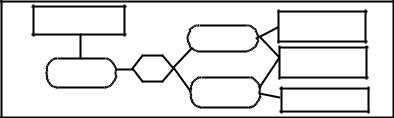
Propagation of Beliefs in a Network of Variables

The evidential diagram becomes a network if one item of evidence pertains to two or more variables in the diagram. Such a diagram is depicted in Figure 2 for a simple case of three variables. Even though the evidential diagram of IT Job Satisfaction model obtained through the RCM approach in the current study is not a network (see Figure 4), we describe the approach of propagating beliefs or m-values through a network of variables for completeness. The propagation of m-values through a network is much more complex and thus we will not go into the details of the propagation process in this chapter. Instead,

Copyright © 2005, Idea Group Inc. Copying or distributing in print or electronic forms without written permission of Idea Group Inc. is prohibited.

Belief Function Approach to Evidential Reasoning in Causal Maps 119

we will briefly describe the process and advise interested readers to refer to Shenoy and Shafer (1990) for the details. Also, Srivastava (1995) provides a step-by-step description of the process by discussing an auditing example.

Basically, the propagation of m-values (i.e., beliefs) through a network of variables involves the following steps. First, the decision maker draws the evidential diagram with all the pertinent variables and their interrelationships in the problem along with the related items of evidence. This step is similar to creating an evidential diagram for the case of a tree-type diagram. Second, the decision maker identifies the clusters of variables over which m-values are either obtained from the items of evidence in the evidential diagram or defined from the assumed relationships among the variables. For example, in Figure 2, the four items of evidence yield the following clusters of variables: {X}, {Y}, {Z}, {X,Y}, and the ‘AND’ relationship defines m-value for the cluster {X,Y,Z}. Thus, in Figure 2, we have the following clusters of variables over which m-values are defined: {X}, {Y}, {Z}, {X,Y}, and {X,Y,Z}.

The third step in the propagation process in a network is to draw a Markov8 tree based on the identified clusters of variables as above. This step is not needed for a tree-type evidential diagram. One can propagate m-values through a tree-type evidential diagram without converting the diagram to a Markov tree. The fourth step is to propagate m- values through the Markov tree by vacuously extending and marginalizing the m-values from all the nodes in the Markov tree to the node of interest. The basic approach to vacuous extension and marginalization remains the same as described earlier through endnotes 5 and 6.

Since the process of propagating m-values in a network becomes computationally quite complex, several software packages have been developed to facilitate this process (see, e.g., Shafer et al., 1988; Zarley & Shafer, 1988; and Saffiotti & Umkehrer, 1991). The software developed by Zarley and Shafer (1988) and Saffiotti & Umkehrer (1991) require programming the evidential diagram in LISP. Also, these software programs do not provide friendly user interfaces. On the other hand the software, “Auditor Assistant,” developed by Shafer et al. (1988) has a friendly user interface and does not require any programming language to draw the evidential diagram. In fact, one can draw the evidential diagram using the graphic capabilities of the software. The evidential diagram drawn by using “Auditor Assistant” looks very similar to the one drawn by hand. The internal engine of the program converts this diagram into a Markov tree and propagates m-values once they are entered in the program. The program can be instructed to evaluate the

Figure 2: Evidential diagram as a network

Copyright © 2005, Idea Group Inc. Copying or distributing in print or electronic forms without written permission of Idea Group Inc. is prohibited.