Добавил:

Upload Опубликованный материал нарушает ваши авторские права? Сообщите нам.

Вуз:

Омский Государственный Технический Университет

Предмет:

[НЕСОРТИРОВАННОЕ]

Файл:

1 / zobaa_a_f_cantel_m_m_i_and_bansal_r_ed_power_quality_monitor

.pdf

Скачиваний:

Добавлен:

30.03.2015

Размер:

32.45 Mб

Скачать

☆

<<< < Предыдущая 1 2 3 4 5 67 / 387 8 9 10 11 12 13 14 15 16 17 18 19 20 21 22 23 24 25 > Следующая >>>

Power Quality Measurement Under Non-Sinusoidal Condition

		FP =	P	≥ FP =	P	(69)
		V	SV	A	SA
			SV		SA
Where	and	are the power factor using the apparent power vector and the arithmetic
definition respectively.

The following expression to calculate the apparent power is proposed in (Goodhue, 1933 cited in Depenbrock, 1992; Emanuel, 1998):

S =	V 2	+ V 2	+ V 2	(70)
S =	ab	bc	ac Ia2 + Ib2 + Ic2	(70)
		3

Conceptually, Eq (70) illustrates that for a given three phase system it is possible to define an equivalent apparent power known as the effective apparent power that is defined as follow:

Se = 3 *Ve * Ie

(71)

Where y are the r.m.s. effective voltage and current values respectively.

Recently, several authors proposed different mathematical representation based on Eq. (71). The most important ones are the one described by the standard DIN40110-2 (Deustcher Industrie Normen [DIN], 2002) and the one developed by the IEEE Working Group (Institute of Electrical and Electronic Engineering [IEEE], 1996) that was the origin of the IEEE Standard 1459-2000 (Institute of Electrical and Electronic Engineering [IEEE], 2000). These two formulations are described next.

3.2 Definition described in the standard DIN40110-2

This method, known as FBD method (from the original authors Fryze, Buchholz, Depenbrock) was developed based on Eq. (71) (Depenbrok, 1992, 1998; Deustcher Industrie Normen [DIN], 2002). It defines the effective values of currents and voltages based on the representation of an equivalent system that shares the same power consumption than the original system.

Then, the effective current can be calculated by the following expression:

IeT =	1 (Ir2	+ Is2	+ It2	+ In2 ) = (I+ )2 + (I− )2 + 4 * (I0 )2
	3
Where , , are the line currents and				the neutral current.
Similarly, the effective voltage is:
	V =	(V2	+ V2	+ V2 ) + (V2				+ V2	+ V2 )	=
	V =	r	s	t			rs	rt	ts	=
	e				12
					12
	= (V )2 + (V )2 +				1	* (V )2
	= (V )2 + (V )2 +					* (V )2
		+		−	4		0
					4

(72)

(73)

This method allows decomposing both currents and voltages into active and non active components. Moreover, it allows distinguishing each component of the total non active term, becoming a suitable method for compensation studies.

48 Power Quality – Monitoring, Analysis and Enhancement

3.3 Definition proposed by the IEEE Standard 1459-2000

This standard assumes a virtual balanced system that has the same power losses than the unbalanced system that it represents. This equivalent system defines an effective line

current	and an effective phase to neutral voltage .
				Ie =	1 (Ir2 + Is2 + It2 + ρ * In2 )	(74)
					3
Where the factor				can vary from 0.2 to 4.
Similar procedure		can be followed in order to obtain a representation for the effective
Similar procedure		=	⁄
voltage	. In this case, the load is represented by three equal resistances conected in a star

configuration, and three equal resistances connected in a delta configuration, the power

relationship is defined by factor				.
Considering that the power	losses are the same for both systems, the effective phase to
		ε = P∆⁄P
neutral voltage for the equivalent system is:
Ve =	3 * (V 2		+ V 2	+ V	2 ) + ε * (V 2 + V2 + V 2 )	(75)
		r	s	t	rs rt ts

				9 * (1 + ε )

In order to simplify the formulations, the standard assumes unitary value of and , then Eq. (74) and (75) can be represented as:

	Ie =	1	(Ir2	+ Is2 + It2	+ In2 )		(76)
		3
Ve =	3 * (V 2	+ V 2 + V 2 ) + (V 2 + V 2				+ V 2 )	(77)
Ve =	r		s	t	rs rt	ts	(77)
				18

These effective current and voltage can also be represented as a function of sequence components:

Ie =	(I+ )2 + (I− )2 + 4 * (I0 )2					(78)
V =	(V )2	+ (V )2	+	1	* (V )2	(79)

e	+	−		2	0

Since one of the objectives of these formulations is to separate the funtamental term from the distortion terms, the effective values can be further decomposed into fundamental and harmonic terms:

			V 2	= V 2	+V	2				(80)
			e	e1	eH
			Ie2	= Ie21 + IeH2						(81)
Where the fundamental terms are:
Ve1 =	3 * (V 2	+ V 2	+ V 2 ) + (V 2			+ V 2	+ V 2	)	(ε = 1)	(82)
	r 1	s1		t1	rs1	rt1	ts1
				18
				18

Power Quality Measurement Under Non-Sinusoidal Condition

Ie1

(Ir21 + Is21 + It21 + In21 )

(ρ =1)

(83)

And the harmonic terms:

V 2 = V 2

− V 2

(84)

IeH2

= Ie2

− Ie21

(85)

Considering these definitions, the effective apparent power can be calculated as follow:

= (3 * V

* I

+ (3 * V

* I

+ (3 * V

* I

)2 + (3 * V

* I

(86)

Where the fundamental term of the effective apparent power is:

Se1 = 3 * Ve1 * Ie1

(87)

The fundamental term can also be represented as a function of active and reactive sequence powers:

(S1+ )2 = (P1+ )2 + (Q1+ )2				(88)
Where:
P+	= 3 *V +	* I+	* cosφ +	(89)
1	1	1	1
Q+ = 3 *V +		* I+ * sinφ +		(90)
1	1	1	1

Then, the square of the fundamental effective apparent power can be represented as the addition of two terms:

Se21 = (S1+ )2 + (SU 1 )2

(91)

Where the term

is due to the system unbalance. Similarly, the non fundamental term

can be represented by:

= (3 * V

* I

)2 + (3 * V

* I

+ (3 * V

* I

(92)

Where the three terms can be represented as a function of the total harmonic distortion, defining the distortion power due to the current as:

DeI = 3 Ve1 IeH = 3 * Se1 * THDI	(93)
The distortion power due to the voltage:
DeV = 3 VeH Ie1 = 3 * Se1 * THDV	(94)
And the effective harmonic apparent power:

50	Power Quality – Monitoring, Analysis and Enhancement
	SeH = 3 VeH IeH = 3 * Se1 * THDV * THDI	(95)

Finally, the harmonic active power can be calculated:

	PH = Vih * Iih * cosφih = P − P1						(96)
	h≠1
	i=r ,s,t
The main features of the formulations proposed by this standard are:				can be separated
from the rest of the active power component. In general			can be neglected since
are small with respect to	, therefore results obtained ,by measuring only this term is
accurate enough. Identify	from the rest of the reactive power componets, it allows to
design the appropriate capacitor bank in order to compensate the power factor shift							.
The non fundamental apparent power		allows evaluating the distortion			severity and
		allows evaluating the distortion				cos

becomes a usefull parameter to estimate the harmonic filter size to compensate the distortion.

Analyzing the apparent power definitions for three phase systems can be observed that the apparent power may have different values depending on the system conditions and the selected definition, being (Eguiluz & Arrillaga, 1995; Emanuel, 1999):

		Sv ≤ Sa ≤ Se				(97)
Similarly observation stands for the power factor values:
FP =	P	≥ FP =	P	≥ FP =	P	(98)

V	SVEC	A	SAVA	e	Se

Method FBD is replaced by the one proposed by the IEEE because it is simpler and is more related to the network parameters

4. Power measurement under non-sinusoidal conditions

The determination of the different power terms such as active power, reactive power, distortion, fundamental component of the positive sequence, and other important parameters ( . . , , , ) are becoming relevant. The power measurement algorithms included in the electronic devices are based on these definitions. Therefore, it is always a concern to implement the most accurate methodology, since errors in power measurement may translate into huge economic losses (Filipsky & Labaj, 1992; Cook & Williams, 1990). In general, these errors are negligible if the system is sinusoidal and balanced; however, this is not the scenario when the system has harmonic or/and unbalanced signals (Cataliotti et al., 2009a, 2009b; Gunther & McGranaghan, 2010).

New technology allows the use of accurate, fast, and low cost measurement systems, however the lack of a unique apparent power definition for unbalanced and distorted systems makes the results of the measurements if not wrong, at least a controversial issue (Morsi & El-Hawary, 2007; Cataliotti et al., 2009a).

In this section, based on the power definitions explained in previous sections and the instantaneous power theory, a methodology to measure power under unbalanced conditions is proposed.

Power Quality Measurement Under Non-Sinusoidal Condition

The algorithm is based on the standard IEEE 1459 – 2000 (Institute of Electrical and Electronic Engineering [IEEE], 2000), the instant power theory, currently used for active filter design, is used for the signal processing phase (Akagi et al, 1983; Herrera & Salmerón, 2007; Watanabe et al., 1993; Akagi et al., 2007; Czarneky, 2006, 2004; Seong-Jeub, 2008) . The Fundamentals of this theory is explained next.

4.1 Instant power theory

A three phase system can be represented by three conductors where the voltage are ,

and the line currents are ,

then, this system can be represented by an equivalent

two

phase system with the following voltages and currents:

vα

and

iα

(99)

= T * vs

= T *

Where is known as the Park transformation matrix:

T =

2 1

−1 / 2 −1 / 2

(100)

3 0

3 / 2

−

3 / 2

Then, the active and reactive power can be calculated as follow:

	p = vα * iα + vβ * iβ			(101)
	q = vα * iβ − vβ * iα			(102)
where:	: instant voltage, direction α,	: instant voltage, direction β,		: instant current
direction α, : instant current, direction		β, : instant active power [W],		: instant reactive
power [VA].
Using matrix notation, the power equation can be represented as:
	p	vα	vβ iα	(103)
	=	−vβ		(103)
	q	−vβ	vα iβ
And the following expression stands:
	P3ϕ = vr * ir + vs * is + vt * it = vα * iα + vβ * iβ			(104)
Where	is the three phase instant power.

These expressions can be extended for a four conductor system; in this case a zero sequence term is needed:

v0vα =vβ

	1 / 2		1 / 2	1 / 2
	1 / 2		1 / 2	1 / 2	vr
2		1	−1 /2	−1 /2	v		(105)
3					s
		0	3 /2 − 3 /2		v
		0	3 /2 − 3 /2		v
						t

52	Power Quality – Monitoring, Analysis and Enhancement
Where:	: Instant zero sequence voltage, : Instant zero sequence current. Similar

expressin can be obtained for the currents. Defining the instant zero sequence power as:

p0 = v0 * i0

(106)

Then, the power vector can be calculated as follow:

p0	v0		0		0	i0
		0	vα
p	=	0	vα		vβ iα
q		0	−v	β	v	i	β
				β	α		β

And the three phase power can be represented by:

P3ϕ = vr * ir + vs * is + vt * it = = vα * iα + vβ * iβ + v0 * i0

From Eq. (106) and (108) the three phase power can be calculated:

P3ϕ = p + p0

(107)

(108)

(109)

Power terms , y can be decomposed using Fourier series and rearranged as a constant power and an harmonic power with a zero mean value:

p = p + p;

			q = q + q;	(110)
			p0 = p0 + p0
Where: :	mean value, : Oscillatory component of , : mean value,			: Oscillatory
component of		, : mean value of	and : Oscillatory component of	. Assuming a
̅		, : mean value of	and : Oscillatory component of	. Assuming a

three phase system distorted, the line current can be represented as a function of the symmetrical components:

∞
ir (t) = 2 * I0n * sin(ωnt + φ0n ) +
n=1
∞
+ 2 * I+ n * sin(ωnt + φ+ n ) +	(111)

n=1

∞

+ 2 * I−n * sin(ωnt + φ− n )

n=1

Same formulae can be obtained for is, it. Similar expressions can be formulated for the voltages. Then, the power equation described in Eq. (110) can be written as a function of symmetrical currents and voltages:

∞
p = 3V+ n * I+ n * cos(ϕ+ n − δ + n ) + 3V−n * I−n * cos(ϕ−n − δ −n )		(112)
n=	1

Power Quality Measurement Under Non-Sinusoidal Condition

∞	∞		+
p =		3V+ m * I+ n * cos((ωm − ωn )t + ϕ+ m − δ + n )	+
m= 1	n= 1
m≠ n

∞	∞		+
+	3V−m * I−n * cos((ωm − ωn )t + ϕ−m − δ −n )		+
m= 1	n= 1
m≠ n
∞	∞			+
+		−3V+ m * I−n * cos((ωm − ωn )t + ϕ+ m − δ− n )		+
m= 1	n= 1
∞	∞
+		−3V−m * I+ n * cos((ωm − ωn )t + ϕ−m − δ + n )
m= 1	n= 1

∞
q = −3V+ n * I+ n * sin(ϕ+ n − δ + n ) + 3V−n * I−n * sin(ϕ−n − δ −n )
n=1
∞	∞		+
q =	−3V+ m * I+ n * sin((ωm −	ωn )t + ϕ+ m − δ + n )	+
m=1	n=1
m≠n

∞	∞		+
+	3V−m * I−n * sin((ωm − ωn )t + ϕ−m − δ −n )		+
m=1	n=1
m≠n
∞	∞		+
+	3V+ m * I−n * sin((ωm − ωn )t + ϕ+ m − δ −n )		+
m=1	n=1
∞	∞
+		−3V−m * I+ n * sin((ωm − ωn )t + ϕ−m − δ + n )
m=1	n=1

(113)

(114)

(115)

		∞
		p0 = 3Von * I0n * cos(ϕ0n − δ0n )		(116)
		n
p0 =		∞		+
p0 =		3Vom * I0n * cos((ωm − ωn )t + ϕ0n −	δ0n )	+
	m= 1	n=1
	m≠ n			(117)
+	∞			(117)
	∞
	−3Vom * I0n * cos((ωm − ωn )t + ϕ0n − δ0n )
m= 1	n= 1

Finally, based on the oscillatory terms, reference (Watanabe et al, 1993) defined the distortion power terms as follow:

H =	2		2	(118)
H =	p	+ q		(118)

4.2 Measurement algorithm evaluation

These previous equations define expressions for real, imaginary and zero sequence power terms as a function of symmetrical components. Based on them, expressions that allow the apparent power calculation considering different conditions are explained next.

54	Power Quality – Monitoring, Analysis and Enhancement

Case 1 - Balanced and sinusoidal system: In this case, the oscillatory, the negative sequence, and the zero sequence terms of both the real and the imaginary power components are zero, therefore the following expression can be proposed for apparent power calculation:

S2 = p2 + q 2 + H 2 = p2 + q 2

(119)

Then the apparent power can be calculated as follow:

S2 = (

3 *V+1 * I+1 )2

= Se2

(120)

Case 2 - Unbalanced load: From Eq. (119), for this case the apparent power is:

2 2

= (3 *V+1 * I+1 )

+ (3 *V+1 * I−1 )

(121)

= 3 *V+1

* (I+1

+ I−1 )

= Se

Case 3 - Unbalanced voltages and currents: In this case, the apparent power is:

= Se2 + 18 * (V+1 *V−1 * I+1 * I−1 ) * cos(ϕ+1 − δ +1 + ϕ−1 − δ −1 )

(122)

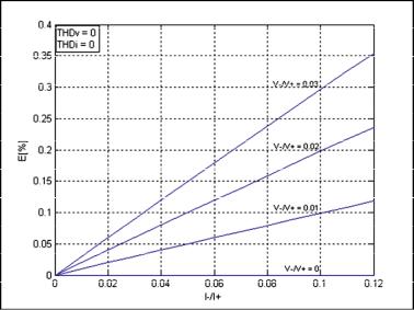
Figure 1 shows the error of

with respect to

as a function of the current unbalance

(

⁄

Each

curve

is parameterized for different values

voltage

unbalance

( = (

)). ). For simplicity, the harmonic distortion, and the phase shift between voltage

and = (

⁄ )

current are zero. The relative error is calculated as follow:

E[%] =

S − Se

(123)

Fig. 1. Measurement error for an unbalanced system

Power Quality Measurement Under Non-Sinusoidal Condition

Case 4 - Balanced and non sinusoidal system: The apparent power for this case can have different formulations depending on where the distortion is present; in the current or in the voltage signals.

a.Distorted current

			∞
		S2	= 9 V+21 I+2n = Se2	(124)
			n=1
b. Distorted voltaje and current
		∞ ∞
S2	= Se2	+ 18 * (V+ n V+ m I+ n * I+ m * cos(ϕ+ n − ϕ+ m − δ + n + δ + m ))		(125)
		n= 1 m= n+ 1

Case 5 - Non sinusoidal system with unbalanced and distorted load: Similar to the previous case, the formulation is different depending on where the distortion is present.

a.Distorted current, sinusoidal voltage

∞

= 9 *V+21 * (I+2n + I−2n ) = Se2

(126)

n= 1

b. Distorted voltaje

S2 = S2 + 18 *

∞ ∞

[

* I

* cos(ϕ

− ϕ

− δ

+ δ

) +

+ n

+ m

+ n

+ m

+ n

+ m

{

+ n

+ m

(127)

n= 1 m= n+ 1

+ I− n * I− m * cos(ϕ+ n − ϕ+ m + δ − n − δ − m )]}

Case 6 - Non sinusoidal system, with unbalanced currents and voltages: This is the most general case where the apparent power, based on Eq.(119) S is determined by the Eq. (128). Eq. (128) is the most general formulation of the apparent power and can be used to calculate the apparent power in all practical cases; all other expressions are a subset of this general one.

S2 = S2

+ 18 *

∞

[

* I

* cos(ϕ

− ϕ

− δ

+ δ

) +

+ n

+ m

+ n

+ m

+ n

+ m

{

+ n

+ m

n= 1 m=n+ 1

+I−n * I−m * cos(ϕ+ n − ϕ+ m + δ − n − δ −m )]} +

+18 *

∞

[

* I

* cos(ϕ

− ϕ

+ δ

− δ

) +

+ n

+ m

−n

−m

+ n

+ m

{ −n

−m

1 m= n+ 1

+I−n * I−m * cos(ϕ− n − ϕ− m − δ −n + δ −m )]} +

+18 *

∞

[

* I

* cos(ϕ

+ ϕ

− δ

) +

(128)

+ n

−m

+ n

− m

+ n

− m

{ + n

−m

1 m= n+ 1

+I+ m * I−n * cos(ϕ+ n + ϕ−m − δ + m − δ −n )]} +

+18 *

∞

[

* I

* cos(ϕ

+ ϕ

− δ

) +

+ n

−m

+ m

− n

+ n

− m

{ + m

− n

1 m= n+ 1

+I+ m * I−n * cos(ϕ+ m + ϕ− n − δ + m − δ − n )]} +

∞

+18 * V+ n *V−n * I+ n * I−n * cos(ϕ+ n − δ + n + ϕ− n − δ −n )

56	Power Quality – Monitoring, Analysis and Enhancement

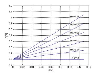
Fig. 2. Measurement error due to voltage and current distortion in an unbalanced system

As an illustrative example, in the case of a three phase system with distortion in both current and voltage signals but with unbalanced load only, the first two terms of Eq. (128) are not zero, then the equation becomes Eq. (125). Figure 2 shows the apparent power deviation with respect to for different values of as a function of . These curves are parameterized for a voltage distortion of 3% and a current distortion of 10%. The figure describes that if THDv is zero, the error is constant regardless of the value of THDi, moreover, the deviation is due to the current and voltage unbalance.

From these results can be seen that the apparent power value is different from the effective apparent power defined by the IEEE only if there is unbalanced or distortion in both current and voltage signals. The maximum relative error can be evaluated from Fig.1 and 2, where the error in the presence of voltage and current unbalance can be determined by the following relationship:

ER% DI * DV * 100	(129)
Similarly for the case of voltage and current distortion:
ER% THDI * THDV * 100	(130)
Therefore, in a general situation, the maximum error is:
ER% (DI * DV + THDI * THDV ) * 100	(131)

These relationships mean that the máximum deviation of S can be evaluated knowing the system condition at the measurement point. In addition to the the formulation presented in this section, the signals can be further processed in order to obtain additional indexes such as the total harmonic distortion, power factor, fundamental power terms, and the active and

<<< < Предыдущая 1 2 3 4 5 67 / 387 8 9 10 11 12 13 14 15 16 17 18 19 20 21 22 23 24 25 > Следующая >>>

Соседние файлы в папке 1

#
30.03.2015471.48 Кб31H03765157.pdf
#
30.03.2015521.43 Кб23IJESIT201303_03.pdf
#
30.03.2015163.97 Кб26kachestvo_elektroenergii_v_energosistemah.pdf
#
30.03.20155.52 Mб30lu_d_dch_ed_an_update_on_power_quality.pdf
#
30.03.2015487.94 Кб37rd_34_20_517_metodicheskie_ukazaniya_po_predotvrasheniyu_fer.doc
#
30.03.201532.45 Mб34zobaa_a_f_cantel_m_m_i_and_bansal_r_ed_power_quality_monitor.pdf