1 / zobaa_a_f_cantel_m_m_i_and_bansal_r_ed_power_quality_monitor

represented mathematically with known parameters are tested. Then two PSCAD/EMTDC simulated disturbance signals due to ground fault and capacitor switching are analyzed using four power quality indices. The sampling frequency for all the transient disturbances is 5 kHz.

4.1 Mathematical transient disturbances

Case1 is low frequency disturbance as voltage sag, swell and interruption that can be expressed mathematically as

where f0 is 50Hz, t1and t2 are the disturbance starting and ending time respectively, α is amplitude change factor: α=-0.1~-0.9 corresponding to voltage sag, α=0.1~0.8 corresponding to swell and -1≤α≤-0.9 corresponding to interruption.

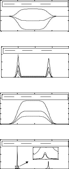
There 30% voltage sag, 50% swell and interruption are constructed using (10) by set α=-0.3, 0.5, -0.9 respectively. The disturbances start at t1=0.1s and end at t2=0.28s. The low frequency disturbance waveforms and S-transform based time frequency distributions are shown is Fig.1. It is can seen that not only fundamental component vary during disturbances occur, but also high frequency component exist at disturbance start and end time.

Fig. 2 shows the four power quality indices of three low frequency disturbances. The IRMS of voltage sag, swell, and interruption in Fig.2(a) is 0.495, 1.061, and 0.0707 respectively during the disturbance occurred, but 0.707 at other time. In Fig.2(b), the IHDR shows two local maximum values corresponding to the start and end time of the three disturbances. The peak values of IHDR for voltage sag, swell, and interruption are 4.63%, 7.93%, 14.6% located exactly at 0.1s and 3.77%, 6.6%, 12.2% at 0.28s. The IWDR of sag, swell and interruption in Fig.2(c) represents the distortion with the value 30%, 50%and 90% from the pure sinusoid, which are consistent with the initial amplitude parameters respectively. With the same local maximum values similar to IHDR, the IAF in Fig.2(d) represents the timevarying instantaneous average frequency for the three disturbances and respective peak values are 51.8Hz, 52.3Hz, 85Hz and 50.5Hz, 50.7Hz, 60Hz.

It can be concluded that these indices effectively represent the transient characteristics of low frequency disturbances. The value of sag amplitude is 0.7 and the corresponding RMS is 0.7 divided by 1.414, which is equal to 0.495. The right results are also represented for voltage swell and interruption; therefore, IRMS accurately represents the RMS varying over time. Compared Fig.2(c) with Fig.2(b), the greater IWDR corresponds with a larger IHDR, this is because there is a larger amplitude change at the start/end time. The IAF shows the similar quantitative relationship corresponding to IWDR and IAF is less deviation from 50 Hz as few high frequency components contained in low frequency disturbances, especially when the disturbances start or end at the zero-crossing point.

In Case2, transient oscillation signal which is a simulation of a capacitor switching event is expressed as

where, f0 and f1 is the fundamental and transient frequency respectively, t1 and t2 are the oscillation starting and ending time, β is the amplitude of exponential function, τ is the decay time coefficient.

Fig. 1. Low frequency disturbances and S-transient based time-frequency distributions: (a) Voltage sag waveform. (b) Time frequency distribution of voltage sag. (c) Voltage swell waveform. (d) Time frequency distribution of voltage swell. (e) Voltage interruption waveform. (d) Time frequency distribution of voltage interruption

Fig. 2. S-transform based power quality indices of voltage sag, swell and interruption: (a) Instantaneous RMS (IRMS). (b) Instantaneous Harmonic Distortion Ratio (IHDR) (c) Instantaneous Waveform Distortion Ratio (IWDR). (d) Instantaneous Average Frequency (IAF)

b)

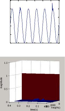
Fig. 3. Transient oscillations and S-transient based time-frequency distribution: (a) Transient oscillation waveform. (b) Time frequency distribution of Transient oscillations

In Fig. 3(a), transient oscillation signal contains two oscillations superposed on the pure sinusoid. The first disturbance is fast oscillation started at t=0.124s (f1 is 1500Hz, β is0.2 and τ is 2.5) and the second disturbance is slow oscillation started at t=0.204s (f1 is 600Hz, β is0.4 and τ is 5). The time-frequency distribution based on S-transform is shown in Fig. 3(b). The IRMS in Fig.4(a) shows two local maximum values 0.754 at 0.124s and 0.795 at 0.204s corresponding to the fast and slow oscillation respectively, which corresponds to the initial amplitude parameter β=0.2 and β=0.4. Moreover, the IRMS of the signal in steady-state time is 0.707 exactly. As there is almost no distortion in fundamental component of the transient oscillation compared with pure sinusoid, that is different from the low frequency disturbance in case 1, the IHDR in Fig.4(b) and the IWDR in Fig.4(c) represent a very similar result with peak value 37.1% and 50.8% at the time oscillations occurred. The IAF represents the deviation of average frequency from f0 and shows peak values 235Hz and 339Hz in Fig.4(d) for the fast and slow oscillation. Though the fast oscillation has a higher frequency component, the slow oscillation induces a greater IAF value than the fast oscillation due to its larger oscillation amplitude and accordingly greater spectral content of high frequency.

Fig. 4. S-transform based power quality indices of transient oscillations: (a) Instantaneous RMS (IRMS). (b) Instantaneous Harmonic Distortion Ratio (IHDR) (c) Instantaneous Waveform Distortion Ratio (IWDR). (d) Instantaneous Average Frequency (IAF)

Concluded from the low frequency disturbances and transient oscillations with known parameters analyzed in the case1 and case2, the results show that the four power quality

indices accurately represent the transient characters of the transient disturbances. IRMS can accurately represent the RMS accommodating the time information. IHDR mainly represents the harmonic component relative to the pure sinusoid fundamental. However, IWDR focuses on the fundamental component distortion of the transient disturbances and also the harmonic distortion. Therefore there is the similar result between IHDR and IWDR when the transient oscillation is analyzed, that is very different from the results of low frequency disturbances. IAF represents the instantaneous average frequency of the transient disturbances and denotes the rated frequency when there is no disturbance occurred.

4.2 PSCAD/EMTDC simulated disturbances

A simple distribution model is built in PSCAD/EMTDC and two transient disturbances: voltage sag and capacitor switching which are two most common disturbances are obtained to illustrate the performance of four power quality indices.

b)

Fig. 5. Voltage sag due to A phase grounded fault: (a) Voltage sag waveform. (b) S- transform based time frequency distribution of voltage sag

A voltage sag caused by A phase grounded fault is simulated and the waveform of A phase voltage is shown in Fig. 5(a). Fig. 5(b) shows the time frequency distribution based on S- transform. The disturbance occurs at 0.082s and ends at 0.313s. The four power quality indices: RMS, IHDR, IWDR and IAF are calculated and a summary of these indices is show in Tab. 1. Similar to the results of the voltage sag in case1, the IRMS is 0.3 and the IWDR is 57.6% during the disturbance occurred. The steady values of IRMS and IWDR are 0.707 and 0. There are also two peaks in the IHDR and IAF corresponding to the start and end time, which are 28.2% and 190Hz at 0.082s and 22.3% and 109Hz at 0.313s respectively. Compared with the voltage sag in case1, this disturbance is not start/end at the zero-crossing point; moreover, there is a larger amplitude change with the IWDR value 57.6%. Consequently, more harmonic content is contained in the disturbance signal, leading to a higher IHDR and a higher IAF.

Table 1. S-transform based four indices of voltage sag

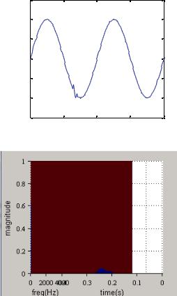
Another disturbance as transient oscillation due to capacitor switching is showed in Fig.6 and the 0.3MVAR capacitor is put into operation at 0.153s. Tab.2. provides the transient peak values and steady values of the four indices. The peak value of IRMS is 0.722 at 0.153s and the peak value of IWDR is 20.1% at the same time that is almost equivalent to the IHDR. The IAF also has a peak value 98Hz when transient oscillation occurred and maintain at 50Hz once the oscillation ended. As the IRMS is a little deviation from the rated value, there is less harmonic content in the disturbance. Accordingly, the value of IHDR, IWDR and IWDR is smaller relative to the disturbance in case2.

Obviously, the two transient disturbances as voltage sag and capacitor switching are characterized well by the four power quality indices. Therefore one can accurately represent the transient information over the time based on the good time-frequency localization properties of S-transform.

Table 2. S-transform based four indices of capacitor switching

b)

Fig. 6. Transient oscillation due to capacitor switching: (a) capacitor switching waveform. (b) S-transform based time frequency distribution of transient oscillation

5. Conclusion

In this chapter, power quality assessment for transient disturbance signals has been carefully treated based on S-transform. The limitations of the traditional Fourier series coefficient based power quality indices, which inherently require periodicity of the disturbance signal, have been resolved by use of time-frequency analysis. In order to overcome the limitations of the traditional power quality indices in analyzing transient disturbances which are non-stationary waveforms with time-varying spectral component, four instantaneous power quality indices based on S-transform are presented. S-transform is shown to be a new time frequency analysis tool producing instantaneous time frequency representation with frequency dependent resolution. In the S-transform domain, new power quality indices: IRMS, IHDR, IWDR and IAF are defined and discussed. The effectiveness of these indices was tested using a set of disturbances represented mathematically and

simulated in PSCAD/EMTDC respectively. The results show that the instantaneous property of transient disturbance can be characterized accurately.

The transient power-quality indices provide useful information about the time varying signature of the transient disturbance for assessment purposes. However, if the timevarying signature can be quantified as a single number, it would be more informative and convenient for an assessment and comparison of transient power quality. The power quality indices proposed in this chapter can be extended to general indices assessment, which should collapse to the standard definition for the periodic case and also be calculable by a standard algorithm that yields consistent results. It is a subject of future research.

6. References

Beaulieu, G.; Bollen, M. H. J.; Malgarotti, S. & Ball, R.(2002). Power quality indices and objectives: Ongoing activates in CIGREWG36-07, Proc. 2002 IEEE Power Engineering Soc. Summer Meeting, pp. 789-794.

Bollen, M. and Yu Hua Gu, I. (2006). Signal Processing of Power Quality Disturbances, Wiley IEEE Press, New Jersey.

CENELEC EN 50160, Voltage characteristics of electricity supplied by public distribution systems.

Chilukuri, M.V. & Dash, P.K.(2004). Multiresolution S-transform-based fuzzy recognition system for power quality events, IEEE Trans. Power Delivery, vol. 19, no. 1, pp.323330.

Domijan, A.; Hari, A. & Lin, T. (2004). On the selection of appropriate wavelet filter bank for power quality monitoring, Int. J. Power Energy Syst., Vol. 24, pp.46-50.

Gallo, D., Langella, R. & Testa, A. (2002). A Self Tuning Harmonics and Interharmonics Processing Technique, European Transactions on Electrical Power, 12(1), 25-31.

Gallo, D., Langella, R. & Testa, A. (2004). On the Processing of Harmonics and Interharmonics: UsingHanning Windowin Standard Framework, IEEE Transactions on Power Delivery, 19(1), 28-34.

Gargoom, A.M., Ertugrul, N. and Soong, W.L. (2005) A comparative study on effective signal processing tools for power quality monitoring, The 11th European Conference on Power Electronics and Applications (EPE), pp.11-4 .

Heydt G. T. & Jewell W. T.(1998). Pitfalls of electric power quality indices, IEEE Trans. Power Delivery, vol. 13, no. 2, pp. 570-578.

Heydt, G. T.(2000). Problematic power quality indices, IEEE Power Eng. Soc. Winter Meeting, vol. 4, pp. 2838-2842.

IEEE Recommended Practice for Monitoring Electric Power Quality. (1995). IEEE Std. 11591995.

IEC 61000-3-6, Assessment of emission limits for distorting loads in MV and HV power systems.

IEC 61000-4-7, General guide on harmonics and interharmonics measurements and instrumentation for power supply systems and equipment connected thereto.

IEC 61000-4-15, Flickermeter, functional design and specifications. IEC 61000-4-30, Power quality measurement methods.

Jaramillo, S.H.; Heydt, G.T. & O’Neill-Carrillo, E. (2000) ‘Power quality indices for a periodic voltages and currents’, IEEE Transactions on Power Delivery, April, Vol. 15, No. 2, pp.784–790.

Lin, T. & Domijan, A.(2005). On power quality Indices and real time measurement, IEEE Trans. Power Delivery, vol. 20, no. 4, pp.2552-2562.

Mishra, S.; Bhende, C.N. & Panigrahi. B.K. (2008) Detection and classification of power quality disturbances using S-transform and probabilistic neural network, IEEE Trans. Power Delivery, vol. 23, no. 1, pp. 280-287.

Morsi, W. G. & EI-Hawary, M. E. (2008). A new perspective for the IEEE standard 1459-2000 via stationary wavelet transform in the presence of non-stationary power quality disturbance, IEEE Trans. Power Delivery, vol. 23, no. 4, pp. 2356-2365.

Shin, Y. J.; Powers, E. J.; Grady, M. & Arapostathis, A.(2006) Power quality indices for transient disturbances, IEEE Trans. on Power Delivery, vol. 21, no. 1, pp.253-261.

Stockwell, R. G.; Mansinha, L. & R. P. Lowe (1996). Localization of the complex spectrum: The S-transform, IEEE Trans. Signal Processing, vol.144, pp. 998–1001.

Ward, D.J. (2001). Power quality and the security of electricity supply, Proceedings of the IEEE, pp.1830-1836.

Voltage sag indices draft 2, working document for IEEE P1564, December 2001.

Zhan, Y.; Cheng, H. Z. & Ding, Y. F.(2005) S-transform-based classification of power quality disturbance signals by support vector machines, Proceedings of the CSEE, vol. 25, no. 4, pp. 51-56.