1 / zobaa_a_f_cantel_m_m_i_and_bansal_r_ed_power_quality_monitor

several decades (Mahdad.b et al., 2007). The solution techniques for the reactive power planning problem can be classified into three categories:

•Analytical,

•numerical programming, heuristics,

•and artificial intelligence based.

The choice of which method to use depends on: the problem to be solved, the complexity of the problem, the accuracy of desired results. Once these criteria are determined, the appropriate capacitor Allocation techniques can be chosen.

The use of fuzzy logic has received increased attention in recent years because of it‘s usefulness in reducing the need for complex mathematical models in problem solving (Mahdad.b, 2010).

Fuzzy logic employs linguistic terms, which deal with the causal relationship between input and output variables. For this reason the approach makes it easier to manipulate and solve problems.

So why using fuzzy logic in Reactive Power Planning and coordination of multiple shunt FACTS devices?

•Fuzzy logic is based on natural language.

•Fuzzy logic is conceptually easy to understand.

•Fuzzy logic is flexible.

•Fuzzy logic can model nonlinear functions of arbitrary complexity.

•Fuzzy logic can be blended with conventional control techniques.

FLC

Fig. 5. Schematic diagram of the FLC building blocks

It is intuitive that a section in a distribution system with high losses and low voltage is ideal for installation of facts devices, whereas a low loss section with good voltage is not. Note that the terms, high and low are linguistic.

3.2 Membership function

A membership function use a continuous function in the range [0-1]. It is usually decided from humain expertise and observations made and it can be either linear or non-linear. The basic mechanism search of fuzzy logic controller is illustrated in Fig. 5.

It choice is critical for the performance of the fuzzy logic system since it determines all the information contained in a fuzzy set. Engineers experience is an efficient tool to achieve a

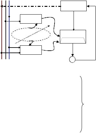
design of an optimal membership function, if the expert operator is not satisfied with the concepetion of fuzzy logic model, he can adjust the parmaters used to the design of the membership functions to adapt them with new database introduced to the practical power system. Fig. 6 shows the general bloc diagram of the proposed coordinated fuzzy approach applied to enhance the system loadability in an Unbalanced distribution power system.

Q P V

Power Flow

Shunt FACTS

Rules I

VregIsvc

Engineer

Experience Rules

Coordination

Vregdes ε

Fig. 6. General schematic diagram of the proposed coordinated fuzzy approach

Where; Qsvcρ , reactive power for three phase.

The solution algorithm steps for the fuzzy control methodology are as follows:

1.Perform the initial operational three phase power flow to generate the initial database (Viρ , Piρ , Qiρ ) .

2.Identify the candidate bus using continuation load flow.

3.Identify the candidate phase for all bus (minViρ ) .

4.Install the specified shunt compensator to the best bus chosen, and generate the reactive power using three phase power flow based in fuzzy expert approach:

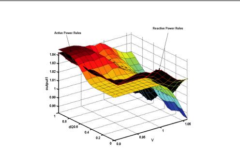
a.Combination Active and Reactive Power Rules. Fig. 7.

Fig. 7. Combination voltage, active and reactive power rules

b.Heuristic Strategy Coordination

-If τ a = τ b = τ c which correspond to the balanced case,

whereτ a ,τ b ,τ c the degree of unbalance for each phase compared to the balanced case. In this case, (Qsvca = Qsvcb = Qsvcc ) .

where τ tot represent the maximum degree of unbalance. the desired degree of unbalance.

Pasy power loss for the unbalanced case. Pbal power loss for the balanced case.

5.If the maximum degree of unbalance is not acceptable within tolerance (desired value based in utility practice). Go to step 4.

6.Perform the three phase load flow and output results.

3.3 Minimum reactive power exchanged

The minimum reactive power exchanged with the network is defined as the least amount of reactive power needed from network system, to maintain the same degree of system security margin. One might think that the larger the SVC or STATCOM, the greater increase in the maximum load, based in experience there is a maximum increase on load margin with respect to the compensation level (Mahdad.b et al., 2007).

In order to better, evaluate the optimal utilization of SVC and STATCOM we introduce a supplementary rating level, this technical ratio shows the effect of the shunt dynamic compensator Mvar rating in the maximum system load, therefore, a maximum value of this factor yields the optimal SVC and STATCOM rating, as this point correspond to the maximum load increase at the minimum Mvar level.

This index is defined as:

i= 1

where: Nsht is the number of shunt compensator Kld: Loading Factor.

QShunt( ρ ) : Reactive power exchanged (absorbed or injected) with the network at phase ρ (a, b, c).

ρ Index of phase, a, b, c.

Step Control

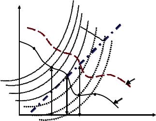
Fig. 8. Schematic diagram of reactive power index sensitivity

Fig. 8 shows the principle of the proposed reactive index sensitivity to improve the economical size of shunt compensators installed in practical network. In this figure, the curve represents the evolution of minimum reactive exchanged based in system loadability, the curve has two regions, the feasible region which contains the feasible solution of reactive power. At point ‘A’, if the SVC outputs less reactive power than the optimal value such as at point ‘B’, it has a negative impact on system security since the voltage margin is less than the desired margin, but the performances of SVC Compensator not violated. On the other hand, if the SVC produces more reactive power than the minimum value ( Qmin ), such as point ‘C’, it contributes to improving the security system with a reduced margin of system loadability, this reactive power delivered accelerates the saturation of the SVC Controllers.

4. Numerical results

In this section, numerical results are carried out on simple network, 5-bus system and IEEE 30-bus system. The solution was achieved in 4 iterations to a power mismatch tolerance of 1e-4.

4.1 Case studies on the 5-bus system

The following cases on the 5-bus network have been studied:

Case1: Balanced network and the whole system with balanced load.

The results given in Table. 1 are identical with those obtained from single-phase power flow programs. The low voltage is at bus 5 with 0.9717 p.u, the power system losses are 6.0747 MW. Neither negative nor zero sequence voltages exist.

Total Power Losses 6.0747 (MW)

Table 1. Three-phase bus voltages for the balanced case. 1

Case2: Balanced network and the whole system with unbalanced load.

4.1.1 Optimal placement of shunt FACTS based voltage stability

Before the insertion of SVC devices, the system was pushed to its collapsing point by increasing both active and reactive load discretely using three phase continuation load flow (Mahdad.b et al., 2006). In this test system according to results obtained from the continuation load flow, we can find that based in Figs. 9, 10, 11 that bus 5 is the best location point.

Loading Factor

Fig. 9. Three phase voltage solution at bus 3 with load Incrementation

Bus 4

Loading Factor

Fig. 10. Three phase voltage solution in bus 4 with load Incrementation

Bus 5

Loading Factor

Fig. 11. Three phase voltage solution in bus 5 with load Incrementation

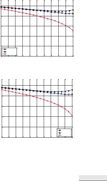
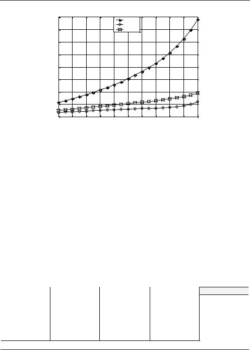
To affirm these results we suppose the SVC with technical values indicated in Table. 2 installed on a different bus. Figs. 9-10-11, show the three phase voltage solution at different buses with load Incrementation. Fig. 12 shows the variation of negative sequence voltage in bus 3, 4, 5 with load incrementation.

Table 2. SVCs data

Bus 3,4,5 -Negative Compnent-

Loading Factor

Fig. 12. Negative sequence voltage in bus 3-4-5 with load incrementation

Case2: Unbalanced Load Without Compensation

Table. 3 shows the three phase voltage solution for unbalanced load, the impact of unbalanced load on system performance can be appreciated by comparing the results given in Table. 3 -4 and Table.1, where small amounts of negative and zero sequence voltages appeared. In this case the low voltage appeared in bus 5 with 0.9599 p.u at phase ‘c’ which is lower than the balanced case, the system power losses are incremented to 6.0755 MW with respect to the balanced case. Table. 4 shows the results of power flow for the unbalanced power system, it can be seen from results that all three phases are unbalanced.

Total Power Loss (MW) 6.0795

Table 4. Three phase bus voltages for the unbalanced case.2: other degree of unbalance

Table 7. SVC at bus 5, step control’18’ (ka=1, kb=0.9, kc=1.1, loading factor=1)

Table 8. SVC at bus 4 and bus 4, 5 (ka=1, kb=0.9, kc=1.1, loading factor=1)

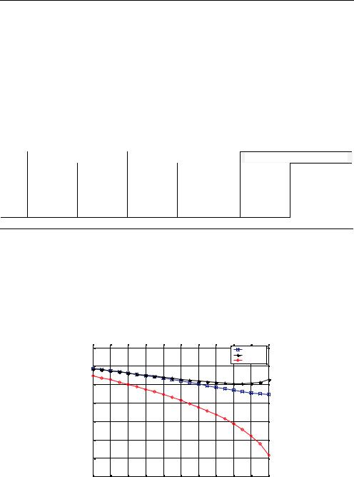
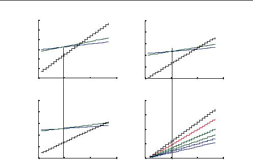
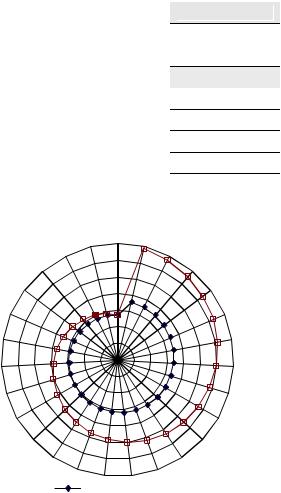
Fig. 16. Voltage profiles for the phase ‘c’ at different SVC installation bus 5, and bus 4