1 / zobaa_a_f_cantel_m_m_i_and_bansal_r_ed_power_quality_monitor

to the substation A busbars. This results from significant differences in the lines lengths and may occur in real systems.

Table 2. Fault in the middle of line (F2)

Table 3. Fault at the origin of line 3 (F3) – line 2 disconnected

Table 4. Fault at the origin of line 1 (F1)

Table 5. Fault at the origin of line 3 (F3)

The method correctness depends to a large extent on the system configuration and this dependence results from the method of operation of the distance protection.

3.8 Vector-space approach [28]

The testing of all these methods show that in cases of asymmetrical voltage dips, they are rather ineffective. Furthermore, al the discussed methods, except the energy based one, require computation of voltage and current phasors for the fundamental-frequency component.

In order to overcome these difficulties vector-space approach is proposed for voltage dip detection. These methods are based on instantaneous voltage and current vectors and their transformation into α,β,0 Clarke’s components. In this way other methods used for voltage dip source detection like the system operating conditions trajectory during the dip (chapter 3.2), the active current based method (chapter 3.7.2), impedance based methods (chapter 3.7.1) and energy based method (chapter 3.4) can be presented in general form.

In Table 6 are presented the generalized methods using a vector space approach.

4. Voltage flictuations

Voltage fluctuations are a series of rms voltage changes or a variation of the voltage envelope. Where only one dominant source of disturbance occurs its identification is usually a simple task. In extensive networks or in the case of several loads interaction, the location of a dominant disturbance source is a more complex process. Where large voltage fluctuations occur in several branch lines it may happen that measurements of flicker severity indices carried out at a power system node, do not indicate disturbing loads downstream the measurement point. The reason is a mutual compensation of voltage fluctuations from various sources.

(a)

(b)

Fig. 25. An example of changes in the flicker severity and the active and reactive power ― phase L1 (diagram in (a))

4.1 Criterion of voltage fluctuations during a fluctuating load operation and after turning it off

The recorded quantities are: the flicker severity Pst and changes in the reactive power Q (also the active power P, if needed) at PCC. The measurements are carried out during the load operation and, where technically possible, after it is turned off. An example records from a steelwork during the arc furnace operation is shown in Fig. 25. Figure shows the results of one week's measurement of the flicker severity Pst, active power P and reactive power Q (phase L1). The dependence of flicker severity values on changes in power, caused by the arc furnace operation, is evident. During the periods the furnace is turned off the reactive power at the measurement point is capacitive due to the presence of fixed capacitor banks. In case several loads are analyzed the measurements have to be carried out during the operation of each load separately.

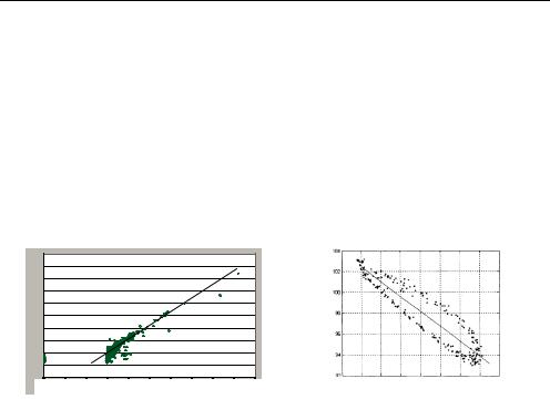
4.2 Correlation of changes in the flicker severity Pst and/or changes in the active and reactive power

The method consists in the analysis of mutual correlation between changes in the reactive power Q (and also the active power P, particularly for low-voltage networks) and the flicker severity value Pst. It allows define the dominant source of disturbance and assess the influence of a change in the load power on the voltage fluctuation in the measurement point. This method can also be applied for assessing the influence of disturbances in individual branches of the network on the total Pst at PCC.

Fig. 26. An example of correlation characteristics of flicker severity Pst and reactive power changes

Fig. 26 shows correlation characteristics of flicker severity Pst and reactive power changes. Characteristic (a) exhibits a strong correlation; it means that a load supplied from the monitored line is the dominant source of voltage fluctuation. In the case (b) the examined load cannot be regarded to be the dominant source.

4.3 Examination of the U-I characteristic slope [23]

Consider two sources of flicker which cause voltage fluctuation at the measurement location PCC: case 1 involves a flicker generating branch at point A and case 2 a similar at point B (Fig. 1). As a result of this flicker caused in the system, the voltage measured at PCC will fluctuate – the current at PCC will show different behaviour for these two cases, similar to criterion used for voltage dip localization.

The frequency of an interharmonic signal depends on operation of the customer's equipment, so it is almost impossible that two devices produce the same interharmonics at the same time. Consequently it is relatively easy to locate the source of interharmonics. This method is fund not to be effective for random flicker source detection.

4.5 Examination of the "voltage fluctuation power"

A conception similar to the method of examining the direction of dominant interharmonics active power flow is presented in [1,3,4]. Similarly to the definition of active power in the time domain there could be introduced so called “flicker power”. Lets define supply voltage and line current in PCC as sinusoidal waveforms with modulated amplitudes as follows

uPCC (t) = (U1 + mU (t)) cos(ω1t) iPCC (t) = ( I1 + mI (t)) cos(ω1t + ϕI ) (43)

where uPCC(t), iPCC(t) are voltage and current waveforms respectively, U1, I1 are magnitudes of the fundamental components, mI(t), mU(t) are amplitude modulation function of current and voltage respectively, ϕI is phase shift of the current with respect to the voltage, ω1 is the angular frequency of the fundamental component.

The human sensitivity to flicker is a function of both modulating frequency and degree of modulation. That means the frequency signals mU (t) and mI (t) must be filtered according to how the human responds to flicker. This is achieved by using the sensitivity filter described in the IEC 61000-4-15. The out signals mUF (t) and mIF (t) indicate how an average

where T is integration time. The flicker power provides two important pieces of information:

•the sign of FP provides information whether flicker source is placed upstream or downstream with respect to the monitoring point.

•when several consumers are investigated, magnitude of FP provides information which outgoing line contributes most to the actual flicker level.

Positive sign of flicker power means the same flow direction as the fundamental power flow. It means that voltage modulation mU (t) is correlated with current modulation mI (t) i.e. decreasing in supply voltage amplitude results in decreasing the load current. Consequently the flicker source is placed upstream with respect to the measuring point. Negative sign of flicker power means the opposite flow direction to the fundamental power flow, and consequently the voltage modulation is negative correlated with current modulation i.e. increasing the current load results in voltage drop. Therefore the flicker source is placed downstream with respect to the measuring point meaning that the load is responsible for voltage variation.

There could be noted, that the method is valid in a specific area of the load reactive power variation.

The method gives correct results under inductive load (the current lags the voltage), and limited capacitive power load (the current waveform leads the voltage waveform). There is also possibility of misinterpretation when a load of constant power demand is considered.

In such a case a voltage drop results in increased current flow. When the reaction is considerable it could be misinterpreted as having the flicker source downstream. The described situations, however, seldom arises in most practical situations.

5. Voltage asymmetry

A three-phase power system is called balanced or symmetrical if the three-phase voltages and currents have the same amplitudes and their phases are shifted by 120° with respect to each other. If either or both of these conditions are not fulfilled, the system is called unbalanced or asymmetrical.

The generator terminal voltages provided to the power system are almost perfectly sinusoidal in shape with equal magnitudes in the three phases and shifted by 120°. If the impedances of the system components are linear and equal for three phases, and if all loads are three-phase balanced, the voltages at any system bus will remain balanced. However, many loads are single-phase and some large unbalanced loads may be connected at higher voltage levels (e.g. traction systems, furnaces). The combined influence of such diverse loads, drawing different currents in each phase, may give rise to the 3-phase supply voltage unbalance. The supply voltage unbalance will then affect other customers connected to the same power network.

To quantify an unbalance in voltage or current of a three-phase system the symmetrical components (Fortescue components) can be used. The three-phase system is thus decomposed into a system of three symmetrical components: direct or positive-sequence, inverse or negative-sequence and homopolar or zero-sequence, indicated by subscripts 1, 2, 0. These transformations are energy-invariant, so for any power quantity computed from either the original or transformed values the same result is obtained. Thus, for active power of a three-phase system we obtain the equation:

The subscripts A, B, C denote the different phases. It should be, however, noted that phase active powers have positive direction (from a source to load). Active powers of the symmetrical components P0 ,P1 ,P2 have no physical meaning and their values depend on the character of the system asymmetry. It can be demonstrated that active power of the direct component has the same direction as the total system active power, but direction of active power of the inverse component depends on the system asymmetry nature. Direction of the inverse component may be used for identifying location of asymmetry source in the system.

measurement

Fig. 28. Circuit diagram for asymmetry source location identification

196 Power Quality – Monitoring, Analysis and Enhancement

In order to examine the method of asymmetry source locating in the analysed diagram the following parameters are taken (in per unit values): U = 100; Rs = Rn = R = 3.536 and Xs = Xn= X = 3.536. Thus, for symmetrical conditions we obtain: I = 10 and U1 = 50.

The following sources of asymmetry in the circuit in Fig. 25 are considered:

Results of the calculation are shown in Table 7. As can be seen, the positive sign of the inverse component active power indicates the system side as the source of asymmetry at the point of measurement (irrespective to voltage or impedance asymmetry), the negative sign of the inverse component active power indicates the load side as the source of asymmetry.

6. Conclusion

In many cases, the quantitative determination of the supplier's and customer's share in the total disturbance level at the point of common coupling (PCC) is also required. Seeking nonexpensive, reliable and unambiguous methods for locating disturbances and assessing their emission levels in power system, not employing complex instrumentation, is one of the main research areas which require the prompt solution. As a result, such research has become an important topic recently.

7. References

[1]Akagi H., Kanazawa Y., Nabae A.: Generalized theory of instantaneous reactive power in three-phase circuit, Proceedings of the International Power Electronics Conference, Tokyo, Japan, 1983, 1375-1386.

[2]Axelberg P.G.V., Bolen M., Gu L.: A measurement method for determining the direction of propagation of flicker and for tracing a flicker source, International Conference CIRED’2005, Turin (Italy), June 2005.

[3]Axelberg P.G.V., Bollen M.,: An algorithm for determining the direction to a flicker source, IEEE Trans. on Power Delivery, 21, 2, 755-760, 2006.

[4]Axelberg P.G.V., Bollen M., Gu L.: Trace of flicker sources using the quantity of flicker power, IEEE Tran. On Power Delivery, 23, 1, 465-471, 2008.

[5]D’Antona G., Muscas C., Sulis S.: Harmonic source estimation: a new approach for the localization of nonlinear loads, 978- 1-4244- 1 770-4/08, 2008 IEEE.

[6]Bollen M.H.J.: Understanding power quality problems – voltage sags and interruptions.

IEEE Press Series on Power Engineering 2000.

[7]Chang G. W., Chen C. I, Teng Y. F.: An application of radial basis function neural network for harmonics detection, 978-1-4244-1770-4/08,2008 IEEE.

[8]Chen C., Liu X, Koval D.,, Xu W., Tayjasanant T.: Critical impedance method - a new detecting harmonic sources method in distribution systems, IEEE Transactions on Power Delivery, 19, 1, January 2004.

[9]Cristaldi L., Ferrero A.: Harmonic power flow analysis for the measurement of the electric power quality, IEEE Tran. Instrum. Meas, 44, 6,1995, pp. 683-685.