1 / zobaa_a_f_cantel_m_m_i_and_bansal_r_ed_power_quality_monitor

then the number of voltage sags recorded are excessive and even exceed the storage capability of the monitor. This increase or decrease in the number of events captured can be explained from the growth of the exposed area with increasing sensitivity of the monitor.

The MRA is defined as the area of the network that is observed from a given monitor position. The exposed area of a bus k is exactly the monitor reach area of a monitor installed at that bus. The ability of the monitor to sense the remote faults is determined by the voltage threshold setting p. The MRA is greater for small voltage changes than for big ones. In other words, one monitor is theoretically able to capture all faults in the network for p equal to 1 pu. Similarly, only solid faults occurring at the monitor position is seen for a threshold p equal to 0 pu.

8.1 Monitor Reach Area (MRA)

The part of the network that is observed by a monitor installed at bus k is thought as an area containing bus k and its electrical neighbourhood. The size of this area depends mainly upon the value of the voltage threshold of the monitor (p). This area is called MRAp for bus k. MRAp is the area of the transmission network, surrounding the monitor position k, for which the monitor is able to capture voltage drops that result in a retained voltage less than or equal to p pu.

The MRAp of bus k is shown as a set of buses. The MRAk,p is the set containing the indices of

the buses within the MRAp of bus k. Using the voltage sag matrix Vdfv, MRAk,p is determined as follows:

The MRA is easily determined from the rows of the voltage sag matrix. A given bus i is part of the MRA of bus k if the voltage at bus k during a fault at bus i is lower than or equal to p pu. Equation (27) allows describing all the monitor reach areas and for any voltage threshold setting of the monitor.

An alternative method to describe the MRAs is by using a binary matrix. For a given voltage threshold setting p, the MRAs are described through an n×n binary matrix in which a 1 in entry (i, j) indicates that bus j belongs to the MRA of bus i. Equation (28) shows this matrix, where vij is the (i, j) entry of the voltage sag matrix.

Once the MRAs for all possible locations are determined the optimization problem is formulated to locate the optimum number of the monitors.

8.2 Optimization problem

Consider a binary variable row vector X of length n indicating if a monitor is needed at bus i. Each element of X, xi, is indicated as follows

The vector X is called Monitor Position Vector (MPV). A given combination of ones and zeros indicates where to install the monitors as expressed in Equation (29).

Fig. 7. Optimal Monitors Emplacements

It is noted that for a given value of the MPV the product of X by the MRAp matrix indicates the number of MRAs that contain each one of the buses i. In order to satisfy the second premise, this product should be greater than or equal to 1 for each bus; meaning that each bus should be in at least one monitor reach area. Let b be a row vector containing ones. The Objective Function (OF) of the optimization problem is formulated as follows

Where xi is the binary decision variable indicating the need for a monitor at bus i; n is the number of potential monitor positions. The right hand side, vector b, defines the level of

redundancy of the monitoring program. A particular value of bi indicates that a fault at the fault position i trigger at least bi monitors. The level of redundancy of the monitoring program is the minimum number of monitors that is guaranteed to trigger on the occurrence of a fault. The letter T over MRAp indicates transposition of the MRA matrix for voltage threshold p.

The voltage sag matrix can be used instead of the MRAp matrix to formulate the optimization problem. This option allows modelling different voltage threshold setting for the monitors. The problem described by Equation (30) is an integer programming optimization problem. A number of algorithms, e.g. Branch and bound Algorithm (BBA) and Genetic Algorithm (GA), have been proposed for solving this type of problem.

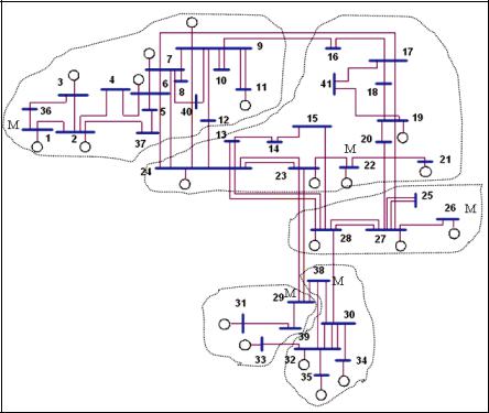
As an example, the optimization method is applied to the sample network of Fig. 3. The BBA algorithm is used to solve the optimization problem. Let the voltage threshold p of the monitors equals to 0.9pu. If all of the faults are considered to be three phase faults, the results of the optimization show that the monitors should be installed at the buses 1, 22, 26, 29, and 38. It is clear that the number of monitors needed to cover the whole system increases with the decrease of the monitor threshold. Fig. 7 shows the optimal monitors emplacements and their reach area.

In Fig. 7, letter M shows the monitor places. The dashed lines also show the reach area of each of the monitors.

9. Conclusion

Power quality monitoring is necessary to characterize electromagnetic phenomena at a particular location on an electric power circuit. In this chapter, the monitoring of voltage sag which is one of the most important power quality phenomena has been discussed. The voltage sag magnitude has been monitored to find the origin of the voltage sag and detect all of the sags in the system.

Voltage sags are determined by fault types, fault impedances, and etc. With respect to the fault type, the shape of the rms voltage evolution shows different behavior. The calculations of all types of faults which may cause the sags have also been discussed in this chapter.

Ideally, a full monitoring program can be used to characterize the performance of entire system, i.e. every load bus should be monitored. Such a monitoring program is not economically justifiable and only a limited set of buses can be chosen for a monitoring program. This has led to the optimal monitoring program which has been proposed in this chapter.

10. References

Baggini, A. (2008). Handbook of Power Quality, Wiley-IEEE Press, ISBN 978-0-470-06561-7, John Wiley & Sons Ltd, West Sussex, England

Bollen, M.H.J. (1999). Understating Power Quality Problems: Voltage Sags and Interruptions,

Wiley-IEEE Press, ISBN 978-0-7803-4713-7, New-York, USA

Casarotto, C. & Gomez, J.C. (2009). Calculation of Voltage Sags Originated in Transmission Systems Using Symmetrical Components, Proceedings of the 20th International Conference on Electricity Distribution (CIRED), Parague, June 8-11, 2009

20 Power Quality – Monitoring, Analysis and Enhancement

Gerivani, Y. ; Askarian Abyaneh, H. & Mazlumi, K. (2007). An Efficient Determination of Voltage Sags from Optimal Monitoring, Proceedings of the 19th International Conference on Electricity Distribution (CIRED), Vienna, Austria, May 21-24, 2007

Grigsby, L.L. (2001). The Electric Power Engineering Handbook, CRC Press, ISBN 978-1-4200- 3677-0, Florida, USA

Mazlumi, K.; Askarian Abyaneh, H. ; Gerivani, Y. & Pordanjani, I.R. (2007). A New Optimal Meter Placement Method for Obtaining a Transmission System Indices, Proceedings of Power Tech 2007 conference, pp. 1165-1169, Lausanne, Switzerland, July 1-5, 2007

Milanovic, J.V.; Aung, M.T. & Gupta, C.P. (2005). The Influence of Fault Distribution on Stochastic Prediction of Voltage Sags. IEEE Transactions on Power Delivery, Vol.20, No.1, (January 2005), pp. 278-285

Moschakis, M.N. & Hatziargyriou, N.D. (2006). Analytical Calculation and Stochastic Assessment of Voltage Sags. IEEE Transactions on Power Delivery, Vol.21, No.3, (July 2006), pp. 1727-1734

Olguin, G. & Bollen, M.H.J. (2002). Stochastic Prediction of Voltage Sags: an Overview,

Proceedings of Probabilistic Methods Applied to Power Systems Conference, Naples, Italy, September 22-26, 2002

Olguin, G. (2005). Voltage Dip (Sag) Estimation in Power Systems based on Stochastic Assessment and Optimal Monitoring, Ph.D. Thesis, Chalmers University of Technology, Göteborg, Sweden

Olguin, G.; Bollen, M.H.J. (2002). The Method of Fault Position for Stochastic Prediction of Voltage Sags: A Case Study, Proceedings of Probabilistic Methods Applied to Power Systems Conference, Naples, Italy, september 22-26, 2002

Salim, F. & Nor, K.M. (2008). Optimal voltage sag monitor locations, Proceedings of the Australasian Universities Power Engineering Conference (AUPEC '08), Sydney, Australia, December 14-17, 2008

2

Wavelet and PCA to Power Quality Disturbance Classification Applying a RBF Network

Giovani G. Pozzebon¹, Ricardo Q. Machado¹, Natanael R. Gomes², Luciane N. Canha² and Alexandre Barin²

¹São Carlos School of Engineering, Department of Electrical Engineering, University of São Paulo ²Federal University of Santa Maria Brazil

1. Introduction

The quality of electric power became an important issue for the electric utility companies and their customers. It is often synonymous with voltage quality since electrical equipments are designed to operate within a certain range of supply specifications. For instance, current microelectronic devices are very sensitive to subtle changes in power quality, which can be represented as a disturbance-induced variation of voltage amplitude, frequency and phase (Dugan et al., 2003).

Poor power quality (PQ) is usually caused by power line disturbances such as transients, notches, voltage sags and swells, flicker, interruptions, and harmonic distortions (IEEE Std. 1159, 2009). In order to improve electric power quality, the sources and causes of such disturbances must be known. Therefore, the monitoring equipment needs to firstly and accurately detect and identify the disturbance types (Santoso et al., 1996). Thus, the use of new and powerful tools of signal analysis have enabled the development of additional methods to accurately characterize and identify several kinds of power quality disturbances (Karimi et al., 2000; Mokhtary et al., 2002).

Santoso et al. proposed a recognition scheme that is carried out in the wavelet domain using a set of multiple neural networks. The network outcomes are then integrated by using decision-making schemes such as a simple voting scheme or the Dempster-Shafer theory. The proposed classifier is capable of providing a degree of belief for the identified disturbance waveform (Santoso et al., 2000a, 2000b). A novel classification method using a rule-based method and wavelet packet-based hidden Markov models (HMM) was proposed bay Chung et al. The rule-based method is used to classify the time-characterized-feature disturbance and the wavelet packet-based on HMM is used for frequency-characterized- feature power disturbances (Chung et al., 2002). Gaing presented a prototype of waveletbased network classifier for recognizing power quality disturbances. The multiresolutionanalysis technique of discrete wavelet transforms (DWT) and Parseval’s theorem are used to extract the energy distribution features of distorted signals at different resolution levels. Then, the probabilistic neural network classifies these extracted features of disturbance type identification according to the transient duration and energy features (Gaing, 2004). Zhu et

al. proposed an extended wavelet-based fuzzy reasoning approach for power quality disturbance recognition and classification. The energy distribution of the wavelet part in each decomposition level is calculated. Based on this idea, basic rules are generated for the extended fuzzy reasoning. Then, the disturbance waveforms are classified (Zhu et al., 2004). Further on, Chen and Zhu presented a review of the wavelet transform approach used in power quality processing. Moreover, a new approach to combine the wavelet transform and a rank correlation is introduced as an alternative method to identify capacitor-switching transients (Chen & Zhu, 2007).

Taking into account these ideas, this chapter proposes the application of a different method of power quality disturbance classification by combining discrete wavelet transform (DWT), principal component analysis (PCA) and an artificial neural network in order to classify power quality disturbances. The method proposes to analyze seven classes of signals, namely Sinusoidal Waveform, Capacitor Switching Transient, Flicker, Harmonics, Interruption, Notching and Sag, which is composed by four main stages: (1) signal analysis using the DWT; (2) feature extraction; (3) data reduction using PCA; (4) classification using a radial basis function network (RBF). The MRA technique of DWT is employed to extract the discriminating features of distorted signals at different resolution levels. Subsequently, the PCA is used to condense information of a correlated set of variables into a few variables, and a RBF network is employed to classify the disturbance types.

2. Proposed classification scheme

Signal

Wavelet

Transform

c9 d1 ,d2 , ,d9

1 10 Feature vector

PCA

RBF

Type of

Disturbance

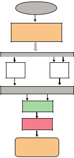
Fig. 1. Diagram of the proposed classification scheme

This section presents the mainframe of the scheme proposed in this paper using the wavelet transform, principal components and neural networks to classify PQ disturbances. The

proposed scheme diagram is shown in Fig. 1. Initially, the input signals are analyzed using the discrete wavelet transform tool, which employs two sets of functions called scaling functions and wavelet functions associated with low pass and high pass filters, respectively. Then, the signal is decomposed into different resolution levels aiming to discriminate the signal disturbances. The output of the DWT stage is used as the input to the feature extraction stage, on which the featuring signal vectors are built. In order to reduce the amount of data, the PCA technique is applied to the feature vector in order to concentrate the information from the disturbance signal and to reduce the amount of the training data used, consequently minimizing the number of input RBF neurons while maintaining the recognition accuracy. Finally, an RBF network is employed to perform the disturbance type classification.

As aforementioned, in the introduction, this work proposes to analyze seven classes of different types of PQ disturbances as follows: Pure sine (C1); Capacitor switching (C2); Flicker (C3); Harmonics (C4); Interruption (C5); Notching (C6); Sag (C7). The databases used for training and evaluation of the proposed system and classification algorithms were performed in Matlab®. The tools used in this approach are presented in sequence.

2.1 The wavelet transform and multiresolution analysis

The DWT is a versatile signal processing tool that has many engineering and scientific applications (Barmada et al., 2003). One area in which the DWT has been particularly successful is transient analysis in power systems (Santoso et al., 2000a, 2000b; Yilmaz et al., 2007), used to capture the transient features and to accurately localize them in both time and frequency contexts. The wavelet transform is particularly effective in representing various aspects of non-stationary signals such as trends, discontinuities and repeated patterns, in which other signal processing approaches fail or are not as effective. Through wavelet decomposition, transient features are accurately captured and localized in both time and frequency contexts.

A wavelet is an effective time–frequency analysis tool to detect transient signals. Its features of extraction and representation properties can be used to identify various transient events in power signals. The discrete wavelet transform analyzes the signal at different frequency bands with different resolutions by decomposing the signal into a coarse approximation and detail information (Chen & Zhu, 2007). This capability to expand function or signal with different resolutions is termed as Multiresolution Analysis (MRA) (Mallat, 1989). The DWT employs two sets of functions called scaling functions, φj,n[t] , and wavelet functions, ψ j,n[t] ,

which are associated with low-pass and high-pass filters, respectively. The decomposition of the signal into the different frequency bands is simply obtained by successive high-pass and low-pass filtering of the time domain signal. The discrete forms of scale and wavelet functions are, respectively, defined as follows.

n

Where cj and dj are the scaling and wavelet coefficients indexed by j, and both functions must be orthonormal.

The wavelet and scaling functions are used to perform simultaneously a multiresolution analysis decomposition and reconstruction of the signal. The former can decompose the original signal in several other signals at different resolution levels. From these decomposed signals, the original signal can be recovered without losing any information. Therefore, in power quality disturbance signals, the MRA technique discriminates the disturbances from original signals, and then they can be analyzed separately (Debnath, 2002). The recursive mathematical representation of MRA is as follows:

version displaying all transient phenomena of the given signal at scale j+1; symbol denotes an orthogonal summation; and n represents the decomposition level.

Since ψ j,n Wj it follows immediately that ψ j,n is orthonormal to φ j,n because all φ j,n Vj are Vj Wj . Also, because all Vj are mutually orthogonal, it follows that the wavelets are orthonormal across scaling. A detailed approach about this theory can be found in (Mallat, 1989; Strang & Nguyen, 1997; Debnath, 2002).

From the engineering point of view, DWT is a digital filtering process in the time domain, by discrete convolution, using the analyses Finite-Impulse-Response (FIR) filters h and g, followed by a down sampling of two. The filter g(k) can generate a detailed version of the signal, while h(k) produces an approximate version of the signal. In the DWT, the resulting coefficients from the low-pass filtering process can be processed again as entrance data for a subsequent bank of filters, generating another group of approximation and detail coefficients.

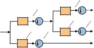
The schematic diagram in Fig. 2 shows two decomposed levels of DWT. The input signal f(t) is split into the approximation cj,k and the detail dj,k by a low-pass and a high-pass filters named h(k) and g(k), respectively. Both, output approximation and detail are decimated by 2. In a practical approach, a DWT depends on:

•the original signal, f(t);

•the low-pass filter, h(k), used;

•the high-pass filter, g(k), used.

There are several families of wavelet functions which contain filters of several supports (filter size). However, in this application, as in (Zhu et al., 2004; Chen & Zhu, 2007), the Daubechie “db4” wavelet was adopted to perform the DWT. As can be seen in (Daubechies,

pair of g. Therefore, from the high-pass filter g the low-pass filter h is obtained, inverting

The coefficients of the “db4” wavelet filters, h and g are presented as follows (Daubechies, 1992).

In practice, the previous filters are the only elements required to calculate the DWT of any signal. As previously mentioned, it is a digital filtering process in the time domain by discrete convolution. In (6) and (7) the relations from the level cj to the next level, cj+1 and dj+1 are given. This relation involves the filters h and g. For specific filter, these equations allow to find the wavelet coefficients using samples of the signal f(t), once the samples are the initial coefficients cj (Mix & Olejniczak, 2003).

Approximation and detail coefficients are down-sampled by 2 in each decomposition level. According to the Nyquist theorem cited in (Mallat, 1989), the maximum frequency of an

original signal f(t) sampled at freqf(t) Hz is (freqf(t)/2) Hz. Therefore, the maximum frequencies freqLevel of signals cj and dj at each resolution level, are given by (8), where freqs is the sampling frequency.

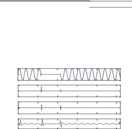
The sampling frequency and amplitude for all types of disturbances considered in this approach are 15.36 kHz (256 samples per period – fundamental frequency of 60 Hz) and 1 p.u., respectively. The wavelet transform is applied to perform a 9-level decomposition of each discrete disturbance signal to obtain the detailed version coefficients (d1 – d9), and the approximated version coefficient (c9). In this experiment, the adopted frequency bandwidths at each decomposition level are shown in Table 1.

Following, it is presented an example of a simple algorithm in MatLab® to demonstrate how the DWT is applied in practice (Mix & Olejniczak, 2003).

%with f as the original signal; N the length of f; and g and h the wavelet filters:

%for one decomposition level, the following is done:

This example code produces decomposed signals (c1 and d1) at level 1, which are the approximated and detailed version of the original signal f, respectively. In this example the signal f contains N samples, but the two derived signals c1 and d1 contain N/2 samples due to down-sampling.

Table 1. Scale to Frequency Range Conversion Based on 60 Hz Power Frequency

Fig. 3. The voltage interruption signal and detail coefficients: first decomposed level (d1), third decomposed level (d3), and fifth decomposed level (d5)