1 / zobaa_a_f_cantel_m_m_i_and_bansal_r_ed_power_quality_monitor

3. Power quality monitoring

The process of the power quality analysis consists of four steps, namely, detection, classification, characterization, and location. Power quality monitoring is used to detect the power quality problems. The monitoring solutions depend on the power quality problems being studied. For example, monitoring of the voltage sags caused by remote faults requires a long-time monitoring. To monitor the power quality problems, the instruments such as multi-meters, oscilloscope, disturbance analyzers, flicker meters, and energy monitors may be used. Some other measuring devices are used for monitoring power quality problems. Although the main purpose of these devices is not the monitoring of the power quality problems, they can be used for this reason. Digital Fault Recorders (DFRs), power meters, and etc. are in this category.

DFR is a monitoring device usually used for monitoring the faults related to the power system disturbances. The DFR is used for metering the bus voltages, line currents, and etc. The high sampling rates (between 6 and 10 kHz) of the DFRs make them possible to record almost all of the events as the transient faults. The DFRs have huge memories for recording and storing the events for a long time.

Monitoring may be used for locating the origins of the power quality disturbances such as voltage sags, harmonics, flickers, and etc. Since the origins of the most voltage sags are the short-circuit faults, the fault locating method and the optimum placement of the monitoring devices are discussed in the rest of this chapter.

4. Voltage sag measurement

Once the fault is cleared, the normal service is restored as soon as possible. The permanent short-circuit faults need to repair the causes of the faults. Therefore, finding the fault location of a permanent fault is necessary to remove the fault cause and to re-energize the network. The fault location problem is usually related to the transmission line for which terminal measurements are available. In this case, the objective of the metering is to find the exact fault location.

The retained voltage during the fault gives the magnitude of a voltage sag. Depending on the type of fault that causes the sag, the voltage during the event may be equal or different in the three phases. According to the symmetrical component classification, two types of symmetrical and unsymmetrical voltage sags are recognized.

Three-phase fault causes balanced voltage sag meaning that the phase voltages during the fault are equal in the three phases. For this kind of voltage sags, only one phase voltage is needed to characterize the magnitude and phase angle of the sag. An unsymmetrical fault may cause the sags with the main drop in one phase or two phases. The equations for voltages during the fault are derived for symmetrical and unsymmetrical faults.

5. Balanced voltage sag

As mentioned above, a three-phase fault causes balanced voltage sag. Consider a network with n buses and its impedance matrix Z. According to the superposition theorem, the voltage during the fault equals the pre-fault voltage at the bus plus the change in the voltage due to the fault. Therefore, the voltage at bus k (= 1, 2, …, n) during a three-phase fault at bus f (= 1, 2, …, n) is given as follows

the fault at bus f. The n2 equations of Equation (3) can be shown in the matrix form as follows

The sag matrix Vdfv contains the during fault voltages (vkf). For example, the row k of Vdfv contains the retained voltages at bus k when faults occur at buses 1, 2, …, f, …, n. Also, the

column f of Vdfv contains the retained voltage at buses 1, 2, …, k, …, n for a fault at bus f. Vpref is the pre-fault voltage matrix. Since the pre-fault voltage at bus k is the same for a fault at any bus, the pre-fault voltage matrix is conformed by n equal columns. V is a matrix

containing the changes in voltage due to faults everywhere. This matrix-based approach is useful for computational implementation of the stochastic assessment.

The voltage changes vkf are calculated by using the impedance matrix. During a threephase fault at bus f, the current injected to the bus f, if, is calculated by

where vpref,f is the pre-fault voltage at the faulted bus f and Zff is the impedance seen looking into the network at the faulted bus f. It is noted that only the positive sequence is needed to

calculate the fault currents.

By obtaining the injected current due to the fault at bus f, the change in voltage at bus k is calculated using the transfer impedance Zkf as follows

The transfer impedance is the voltage that exists on bus k when bus f is driven by an injection current of unity. Replacing vkf from Equation (6) in Equation (3) results in

Equation (7) is simplified by neglecting the load, which allows taking the pre-fault voltages equal to 1p.u. This equation shows that the voltage change at a bus k due to a three-phase fault at bus f is given by the quotient between the transfer impedance and the driven point impedance at the faulted bus. The positive sequence impedance matrix Z is a diagonal dominant full matrix for a connected network. This means that every bus is exposed to sag due to fault everywhere in the network. However, the magnitude of the voltage drop depends on the transfer impedance between the observation bus and the faulted point. Therefore, the load buses are not seriously affected by faults located far away in the system. The voltage change also depends on the driving impedance at the faulted bus. The driving impedance determines the weakness of the bus.

10 Power Quality – Monitoring, Analysis and Enhancement

The pre-fault voltage at the load bus k, vpref,k, only contains the positive-sequence component and is equal to the pre-fault voltage in phase A. The during-fault sequence voltages at bus k

are given by Equation (13).

After transforming the equations into the phase components, Equation (14) is derived.

From Equation (13), it is clear that the phase voltages at bus k do not contain a zero sequence component if the zero sequence of the transfer impedance Zkf is null. The zero sequence of the transfer impedance is null when the load and the fault buses are at different sides of a transformer with delta winding. Equation (14) gives the retained phase voltage for a general case. The negative sequence impedance matrix is usually equals to the positive sequence impedance matrix. If the zero sequence voltage can be neglected, Equation (14) is simplified as Equation (15).

Equation (15) shows that the retained phase voltages at the observation bus is calculated using a balanced short circuit algorithm by adding a fault impedance equal to half of the value of the zero sequence driving point impedance at the faulted bus. This means that a SLG fault is less severe than a three phase fault in regard to the depression in the voltage seen at the load bus. Due to the zero-sequence impedance, the faulted phase shows a smaller drop compared to a sag originated by a three-phase fault.

6.2 Voltage changes in Line to Line (LL) fault

For a LL fault, only the positive and the negative sequence networks are considered to analyze the fault. There is no zero sequence current and voltage. In this type of fault, the positive sequence current at the fault location is equal in magnitude to the negative sequence current, but in opposite direction. Equation (16) gives the injected currents in the sequence networks.

The change in positive and negative sequence voltages are given by Equation (17). There is no zero sequence voltage change.

The retained phase voltages are obtained by adding the pre-fault voltage to Equation (17). Equation (18) shows transforming the sequence components into the phase components.

If the positive sequence impedance matrix is equal to the negative sequence impedance matrix, Equation (18) is simplified as indicated in Equation (19).

where 1 is a matrix full of ones and such that its dimension is equal to the dimension of Z.

The square n × n matrix Vdfv contains the sags at each bus of the network due to faults at each one of the buses. The during fault voltage at a general bus j when a fault occurs at that

bus is contained in the diagonal of Vdfv and is zero for a solid three phase fault. Off-diagonal

elements of Vdfv are the sags at a general bus k due to a fault at a general position f. Hence, column f contains the during-fault voltages at buses 1, 2, …, f,…, n during the fault at bus f.

This means that the effect, in terms of sags, of a fault at a given bus of the system is contained in columns of the voltage sag matrix. This information is usually presented on the single line diagram of the power system and it is called affected area. A sample n ×n sag matrix is shown as follows

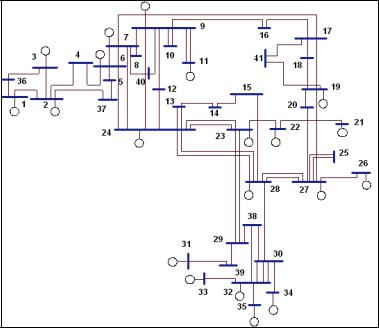
In this chapter, a real sample network is used for description of the voltage sag matrix. Fig. 3 shows a 41-bus 230-kV of Tehran Regional Electric Company in Iran.

Fig. 3. Single line diagram of a 230 kV real case study

Applying Equation (23), it is found the during fault voltages for the 41 buses due to the faults on each one of the 41 buses. Equation (26) shows the resulting voltage sag matrix. It is seen that column 34 of the sag matrix contains the during fault voltages at each one of the 41 buses when a three-phase fault occurs at bus 34. Column 34 of the sag matrix contains the information to draw the affected area of the system due to a fault at bus 34.

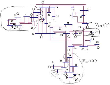
Fig. 4. Affected areas for three-phase fault at buses 34 and 21

The affected area contains the load buses that present a during fault voltage lower than a given value due to a fault at a given bus. In Fig. 4, three affected areas are presented for

three-phase faults on the middle of the line 1-2 and the buses 21 and 34. The areas enclose the load buses presenting a sag more severe than a retained voltage of 0.9 p.u. If the threshold is less than 0.9, the areas are smaller than the areas shown in Fig. 4. Only the original impedance matrix of positive sequence of the system is used to build the exposed areas. Faults on lines are more frequent than fault on buses of the system, however faults on buses cause more severe sags in terms of magnitude and therefore are considered for building the affected areas. In the rest of this chapter, only faults on the buses are to be considered.

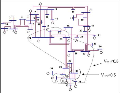
The exposed area (area of vulnerability) is contained in rows of the voltage sag matrix and as in the case of the affected area can be graphically presented on the single line diagram. Fig. 5 presents the exposed area of bus 32. The exposed area encloses the buses and line segments where faults cause a sag more severe than a given value. In Fig. 5, the 0.5 p.u. exposed area of bus 32 contains buses 30 and 32. Similarly, the 0.8 pu exposed area for bus 32 contains all the buses where faults cause a retained voltage lower than 0.8 pu. Fig. 5 suggests that the exposed area is a closed set containing buses.

Fig. 5. Exposed area of bus 32 for three-phase faults

Unsymmetrical faults can also be considered to define the exposed area of a sensitive load. Positive, negative, and zero sequence impedance matrices are needed to perform the calculations.

To show the exposed areas for symmetrical and unsymmetrical faults, the exposed areas of a three phase fault and a SLG fault at bus 35 are illustrated in Fig. 6. In this figure, the 0.8 pu

SLG fault exposed area of bus 35 contains buses 30 and 32. Also, the 0.8 pu three phase fault exposed area contains buses 30, 32, and 38. The SLG fault exposed area is almost coincident with the three phase fault exposed area, however, a bit smaller.

Fig. 6. Exposed area of bus 35 for SLG and three-phase faults

It is noted that the exposed area is also the area for which a monitor, installed at a particular bus k, is able to detect faults. For example, if a monitor is installed at bus 30 and the boundary for sag recording is adjusted to 0.8 pu, then the monitor is be able to see the faults in the 0.8 pu exposed area of bus 30. When referring to power quality monitors the exposed area is called Monitor Reach Area (MRA). In the next section, the way of optimal locating of the monitors is described to monitor all of the faults in the system.

8. Optimal placement of voltage sag monitors

In order to find optimal monitor locations for a monitoring program, the following two premises are considered:

•A minimum number of monitors should be used.

•No essential data concerning the performance of load buses in terms of sags should be missed.

The number of voltage sags recorded at a substation during a given monitoring time depends upon the critical threshold setting of the power quality monitor. It is considered the threshold level as the voltage p in pu at which the monitor starts recording. If the threshold is set too low (e.g., 0.5 pu), then the monitor do not capture an important number of disturbances. On the other extreme, if the threshold (p) is set high (e.g., 0.9 pu or higher)