

Lecture no. 24. Double integral
POINT 1. DOUBLE INTEGRAL
POINT 2. EVALUATION OF A DOUBLE INTEGRAL IN CARTESIAN COORDINATES
POINT 3. IMPROPER DOUBLE INTEGRAL. POISSON’S FORMULA
Point 1. Double integral
Def. 1. Let a
function of two variables
![]() be given in a some domain D
of the
-plane
(fig. 1).
be given in a some domain D
of the
-plane
(fig. 1).
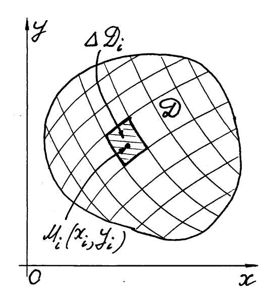 1.
We divide the domain into n
parts
1.
We divide the domain into n
parts
![]() with
areas
with
areas
![]() and diameters
and diameters
![]() .
.
2. We take arbitrary point
![]() in every part
in every part
![]() ,
find the value of the function at this
point and multiply it by the area
of
.
,
find the value of the function at this
point and multiply it by the area
of
.
3. We add all these products
![]() Fig. 1 and get an integral sum
Fig. 1 and get an integral sum
![]() .
.
4. Let
![]() and
.
If there exists the limit of the integral sum
and
.
If there exists the limit of the integral sum
![]() ,
then this limit is called the double integral of the function
over the domain D
and is denoted by
,
then this limit is called the double integral of the function
over the domain D
and is denoted by
![]() ( 1 )
( 1 )
We can consider the
double integral as the sum of elements
![]() where dS =
dxdy is an
element of the area.
where dS =
dxdy is an
element of the area.
Theorem 1 (existence of a double integral). If a function is continuous in a domain D then its double integral over D exists.
It is evident that for
![]() a double integral gives the area of the domain D,
a double integral gives the area of the domain D,
![]() .
( 2 )
.
( 2 )
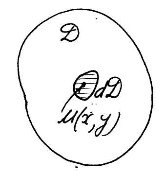
Mechanic sense of
a double integral. If
![]() is the surface density of a plate
is the surface density of a plate![]() ,
then its mass equals the next double integral
,
then its mass equals the next double integral
![]() ( 3 )
( 3 )
■An element of the mass
![]() ;
;
it
is the mass of the element
![]() with the area
and with a constant surface density
with the area
and with a constant surface density
![]() (fig. 2). Sum of all
these elements
gives the mass of the plate which is
re-
Fig. 2 presented by a double integral
(3).■
(fig. 2). Sum of all
these elements
gives the mass of the plate which is
re-
Fig. 2 presented by a double integral
(3).■
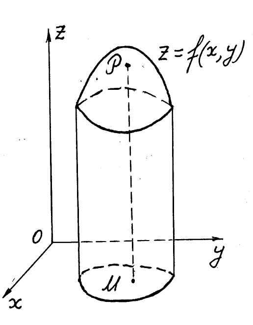
 Def.
2. A cylindrical body [a curvilinear
cylinder] is called a body bounded:
Def.
2. A cylindrical body [a curvilinear
cylinder] is called a body bounded:
a) above by a surface
![]() ;
;
b) below by a domain D of the xOy-plane;
c) aside by a
cylindrical surface with the generatrix parallel to![]() -axis
and the diréctrix which is the boundary of
the domain
Fig. 3 Fig. 4
D
(fig. 3).
-axis
and the diréctrix which is the boundary of
the domain
Fig. 3 Fig. 4
D
(fig. 3).
Geometric sense of a double integral. The volume of a cylindrical body equals the double integral
![]() .
( 4 )
.
( 4 )
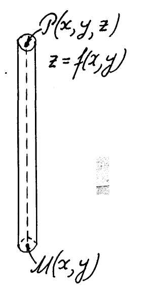
■An element of the volume
![]()
is
the volume of a right circular cylinder with the base
of the area
and the height
![]() (fig. 4). The volume of a cylindrical body is the sum of all these
elements and is represented by the double integral (4).■
(fig. 4). The volume of a cylindrical body is the sum of all these
elements and is represented by the double integral (4).■
Properties of a double integral are the same as for a definite integral.
For example:
1 (linearity). For
any functions
![]() and any constants
and any constants
![]() .
.
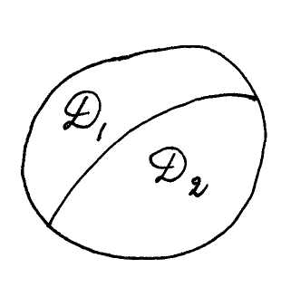 2
(additivity). If a domain is divided into
two disjoint parts
2
(additivity). If a domain is divided into
two disjoint parts
![]() ,
,
![]() (fig. 5), then
(fig. 5), then
![]() .
Fig. 5
.
Fig. 5
Point 2. Evaluation of a double integral in cartesian coordinates
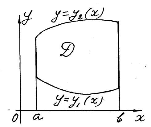 Def.
3. A domain D
is called a domain of the first type
if it is bounded (see fig. 6):
Def.
3. A domain D
is called a domain of the first type
if it is bounded (see fig. 6):
a) from the left by a straight line ;
b) from the right by a straight line ;
c) below by a line
![]() ;
;
d) above by a line
![]() ,
Fig. 6
,
Fig. 6
![]() .
.
A double integral over a domain of the first type is calculated by a formula
 .
( 5 )
.
( 5 )
 Correspondingly
to this formula we integrate at first with respect to y
from
Correspondingly
to this formula we integrate at first with respect to y
from
![]() to
to
![]() ,
that is calculate an inner integral
,
that is calculate an inner integral
 ,
Fig. 7 and then we integrate the result
with respect to x
from a to
b.
,
Fig. 7 and then we integrate the result
with respect to x
from a to
b.
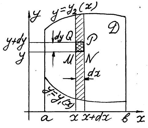
■We’ll prove the formula (5) proceeding from
the mechanic sense of a double integral.
Let the integrand
![]() be the surface density of a plate, defi-ned by the figure
be the surface density of a plate, defi-ned by the figure
![]() (fig. 6). Hence the
mass of the plate equals the double integral
(fig. 6). Hence the
mass of the plate equals the double integral
![]() .
.
Now we’ll find the same mass by the other way
and compare the results. The mass of the element
![]() of the plate between
of the plate between
![]() and
and
![]() (fig. 7) equals
(fig. 7) equals
![]() .
Adding all such the masses from
.
Adding all such the masses from
![]() to
to
![]() we find the mass of the hatched strip (fig. 7), namely
we find the mass of the hatched strip (fig. 7), namely
 .
.
Adding finally the masses of all such the strips from to we find the mass of the whole plate that is
 .
.
Comparing of two results of the mass calculating proves validity of the formula (5).■
Note 1. Integral with respect to x from a to b is called that exterior [external]. The right side of the formula (5) is called the repeated integral.
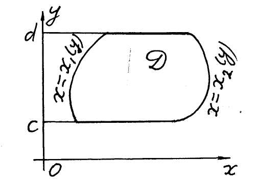
Def. 4. A domain D is called a domain of the se-cond type if it is bounded (see fig. 8):
 a)
below by a straight line
a)
below by a straight line
![]() ; b)
above by a a straight line
; b)
above by a a straight line
![]() ; c)
from the left by a line
; c)
from the left by a line
![]() ;
d) from the right by a line
;
d) from the right by a line
![]() ,
,
![]() .
.
Fig. 8 The double integral over a domain D of the se-cond type is calculated by a formula
 .
( 6 )
.
( 6 )
At first we calculate an inner integral
 ,
,
that
is integrate with respect to x from
![]() to
to
![]() ,
and then we integrate the result with respect to y
from c
to d.
,
and then we integrate the result with respect to y
from c
to d.
 ■Prove
this formula yourselves.■
■Prove
this formula yourselves.■
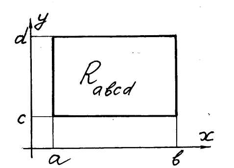
Ex. 1. Let a domain of integration is a rectangle
![]()
with the sides parallel to Ox-, Oy-axes (fig. 9). The rec-tangle is the domain of the first and second types, there- Fig. 9 fore we can use both formulas (5) and (6),
 .
( 7 )
.
( 7 )
The formula (6) means that in the case of the
rectangle
![]() we can integrate in any order. But one of orders of integration can
lead to easier calculations than the other one.
we can integrate in any order. But one of orders of integration can
lead to easier calculations than the other one.
Ex. 2. Find the mass of a plate
![]() (fig. 10)
(fig. 10)
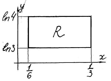 if
the surface density of the plate equals
if
the surface density of the plate equals
![]() .
We find the mass by the formula (3). A domain of
integration R is
a rectangle with the sides parallel to Ox-,
Oy-axes.
Using the formula (7) we get
Fig. 10
.
We find the mass by the formula (3). A domain of
integration R is
a rectangle with the sides parallel to Ox-,
Oy-axes.
Using the formula (7) we get
Fig. 10

![]() .
.
The other order of integration isn’t well (verify!).
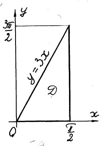 Ex.
3. Evaluate by two ways the integral
Ex.
3. Evaluate by two ways the integral
![]() if the domain D is
defined by inequalities
if the domain D is
defined by inequalities
![]() (fig. 11).
(fig. 11).
The domain D is that of the first and second types.
The first way. We consider D as a domain of the first type,
![]() ,
Fig. 11 that is D is
bounded
,
Fig. 11 that is D is
bounded
a) from the left by the straight line
![]() ;
;
b) from the right by the straight line
![]() ;
;
c) below by the line
![]() ;
;
d) above by the line
![]() .
.
Using the formula (5) we have


In the second way we treat D as a domain of the second type,
![]() ,
,
that is D is bounded
a) below by the straight line ;
b) above by the straight line
![]() ;
;
c) from the left by the line
![]() ;
;
d) from the right by the line .
Therefore with the help of the formula (6) we write
 .
.
Fulfill evaluation of the integral yourselves.
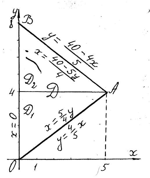
Ex. 4. Set the limits of integration in a double
integral over a triangular domain D with
the vertices
![]()
Fig. 12 (fig. 12)
At first we compile the equations of the straight lines OA and AB.
OA:
![]()
AB:
![]()
![]() .
.
The first way. The domain D
is that of the first type because of
it’s bounded from the left by a straight line x
= 0, from the right by a straight line
x = 5,
below by a line
![]() ,
above by a line
,
above by a line
![]() hence on the base of the formula (5)
hence on the base of the formula (5)
 .
.
The second way. To apply the formula (6) we divide
the domain D into
two domains
![]() of the second type by a straight line y
= 4 (fig. 12). If we describe them by
two double inequalities, namely
of the second type by a straight line y
= 4 (fig. 12). If we describe them by
two double inequalities, namely

 we’ll
get
we’ll
get
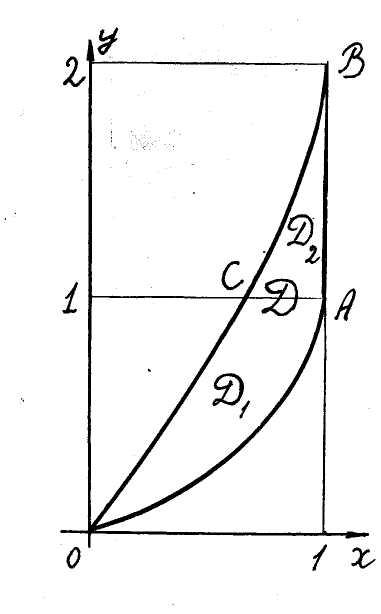
Ex. 5. Evaluate the double integral
![]()
Fig. 13 over the domain
![]() (fig. 13).
(fig. 13).
The
domain D
is that of the first type. It can be divided into two domains of the
se-cond type
![]() by the straight line
by the straight line
![]() (fig. 13),
(fig. 13),
![]() ,
,
![]() ,
,
![]() .
.
The integral in question equals the sum of two integrals. It’s well to calculate
the
first one over the domain D and
the second one as the sum of integrals over
![]() and
and
![]() .
.

![]() .
.