

Point 2. Arс length
Let ˘ be an arc of some curve, and it’s necessary to find its length.
T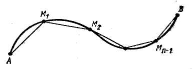 he
first method. We divide the arc ˜AB
into n
parts by points
he
first method. We divide the arc ˜AB
into n
parts by points
![]() and inscribe the poly-gonal line
and inscribe the poly-gonal line
![]() in ˘AB (fig.
15). Let
Fig. 15
in ˘AB (fig.
15). Let
Fig. 15
![]() ( 12 )
( 12 )
is
the perimeter of the polygonal line and
![]() .
If there exists the limit
.
If there exists the limit
![]() (
13 )
(
13 )
it is called the length of the arc ˘AB.
Let an arc ˘ of a curve is determined in Cartesian coordinates by an equation
( 14 )
on
a segment
![]() ,
and
,
and
![]() be the coordinates of the point
be the coordinates of the point
![]() ,
,
![]() .
In this case
.
In this case
![]() ,
,
and
by Lagrange theorem there is a point
![]() such that
such that
![]() .
.
Denoting
![]() we get
we get
![]() and therefore
and therefore
![]() .
.
Passage to the limit gives the desired arc length as a definite integral from a to b,
![]() .
( 15 )
.
( 15 )
The arc length L exists if a function is continuous with the first derivative on the segment .
The second method. We find at first an element (or
the differential)
![]() of
the desired arc length and then the arc length as the sum of all the
elements.
of
the desired arc length and then the arc length as the sum of all the
elements.
By Pythagorean theorem
![]() and
and
![]() .
( 16 )
.
( 16 )
For an arc ˘ determined by an equation (14)
![]() ,
,
and the sum of all the elements from a to b leads to the same formula (15).
If an arc ˘ of a curve is determined parametrically by equations
![]() ,
( 17 )
,
( 17 )
we have from (16)
![]() ,
,
and therefore
![]() .
( 18 )
.
( 18 )
If an arc ˘ of a curve is given in polar coordinates by an equation
![]() ( 19 )
( 19 )
we pass to parametrical equations of the arc
![]() ( 20 )
( 20 )
and apply the formula (18). Since
![]()
![]()
the formula (18) gives
![]() .
( 21 )
.
( 21 )
Ex. 10. Find the arc length of a curve
![]() for
for
![]() .
.
By virtue of the formula (15) we have
![]()
![]()
Ex. 11. Find the length of the loop of the curve
![]() (fig. 11).
(fig. 11).
By the formula (18)

![]() .
.
Ex. 12. Find the length of the cardioid (fig. 13).
With the help of the formula (21)
![]()
![]() .
.
Ex. 13. Find the length of an ellipse
![]() .
.
Parametrical equations of the ellipse
![]() and
by the formula (18)
and
by the formula (18)
![]() .
.
We can find only approximate value of L for given values of a and b because of a pri-mitive of the integrand is inexpressible in terms of elementary functions.
Ex. 14. Prove that the length of Bernoulli lemniscate (fig. 14) can be represented by the next integral
![]() .
.