262 ELECTRICAL CONDUCTIVITY OF PARTIALLY IONIZED PLASMA

of a term proportional to the next degree of density. On introducing the pair correlation function of atoms g(r) and making transformations in (6.18), the mean square ofthe scattering amplitude per atom may be represented as

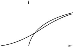
where S(k) is the structure factor of the medium.

The expression for the collision frequency has the form

where q(v, θ) is the di erential cross–section of electron–atom scattering. Figure 2.22 shows the structure factor of rubidium. One can see that it is a nonmonotonic function of k and thermodynamic parameters of the medium. Therefore, the effect of correlations on mobility may vary considerably. Depending on the conditions, the mobility may decrease or increase, as compared with the mobility calculated in an ideal–gas approximation.

Podlubnyi et al. (1988) treated the coe cient of electrical conductivity of a multicomponent plasma. The electron scattering probability was averaged over the multicomponent system of scattering centers. The resultant collision fre-

number the sorts of particles, na and nb denote the concentration, and fa and fb are the scattering amplitudes.

In the Debye–H¨uckel approximation, the ion–ion structure factor is given by expression (5.6). Formula (6.20) may be used to calculate the coe cient of electrical conductivity in a plasma, in which ions with di erent charge numbers are present.

6.3Electrical conductivity of nonideal weakly ionized plasma

6.3.1The density of electron states

In Chapter 4 we have treated the conditions in dense vapors of metals, when ions occur in clusters. This a ects considerably the ionization equilibrium. As to the electrons, they remain free, that is, they are conduction electrons. However, a di erent situation is possible. If the density is high, and the energy of electron attachment to atom is su ciently high, the fluctuations of the medium density

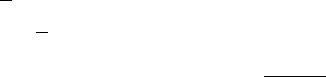
Fig. 6.6. Qualitative dependencies of ρ(E) and ρ0(E).

may cause deep potential wells. An electron is captured in such wells and making a transition to the negative-energy region stabilizes this fluctuation of density. An electron cluster emerges and, because it is characterized by low mobility, the electron is said to be localized.

The e ect of self–trapping of electrons is characteristic of dense disordered systems; see, for example, Lifshitz (1965); Ziman (1979); Shklovskii and Efros (1984); Hernandez (1991). It is also possible that the electrons are localized in dense vapors of mercury (Khrapak and Iakubov 1981). The distribution of electrons in positive and negative energies is defined by the density of electron states in a dense medium. The main question, which arises, is as follows: the electrons of what energy have su cient mobility to be regarded as conduction electrons? The theory may hardly provide an answer to this question. It permits the development of only rather crude models. The density of electron states ρ(E) defines the electron concentration in the given energy range

where µe is the chemical potential of the electronic gas. In an ideal gas,

It is well known that in a dense medium due to atom density fluctuations ρ(E) may qualitatively di er from ρ0(E). First, the continuous spectrum boundary shifts through the value of mean field. In addition, there emerges a “tail” of the density of states ρ(E), extending to the region of forbidden states with negative energy, Fig. 6.6. The states of the remote tail ρ(E) correspond to electrons trapped in heavy clusters. At the same time the electrons with relatively low absolute values of negative energy may have a considerable mobility.

264 ELECTRICAL CONDUCTIVITY OF PARTIALLY IONIZED PLASMA

At present, one cannot regard all of the emerging problems as solved even on the qualitative level. The quantum e ects are especially di cult to describe. Much simpler is the classical electron behavior in a dense medium.

The density of states of a classical electron placed in a potential field U (r) generated by scatterers whose number is equal to N is defined by the expression

where

N

E(r, p) = p2/2m + U (r); U (r) = V (r − Ri).

i=1

Here, r and p denote the electron coordinate and momentum, Ω is the system volume, and the averaging is performed over all possible scatterer configurations. For an arbitrary function Y (R1, R2, . . . , RN ) its mean value is given by

where Va(Ri − Rk) is the energy of interaction between the ith and kth atoms. In a rarefied gas, the potential energy of an electron in the atomic field U (r) can be ignored. Then, it follows from Eq. (6.23) that ρ(E) = ρ0(E). In a dense gas, the calculation of ρ(E) is related to the concrete form of the potential V (r). The simple result can be obtained by including only the most probable fluctuations of the field U described by the Gaussian approximation. Performing

an integration over momenta in Eq. (6.23) we get

The averaging over all atomic configurations in Eq. (6.24) can be replaced by averaging over a random field distribution P (U ). Then,

Let nV be the magnitude of the mean field U and nW0 its dispersion n V 2(r)dr, where n = N/Ω is the density of scatterers. For high negative energies (E − nV )2 nW0 we then have

Consequently, deep in the “tail” ρ(E) decreases exponentially. In the region of renormalized zero, ρ(E) is finite,

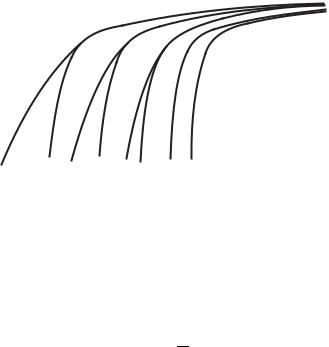
Fig. 6.7. Electron state density ρ(ε) as a function of relative electron energy ε for correlated (solid curves) and uncorrelated (dashed curves) scatterers (Lagar’kov and Sarychev 1975). Numbers correspond to di erent atomic densities: 1.33 · 1022 cm−3 (1); 8.3 · 1021 cm−3 (2); 4.8 · 1021 cm−3 (3); 2.4 · 1021 cm−3 (4); 1.05 · 1021 cm−3 (5).

Given high positive energies, ρ(E) assumes the regular root dependence but with an energy shift, ρ(E) = ρ0(E −nV ). Such dependence of ρ(E) is proper for strongly nonideal disordered systems.

It should be mentioned that Eq. (6.27) cannot correctly describe the ρ(E) tail if the depth of the electron–atom interaction potential is comparable with or exceeds the temperature. In such cases, the ρ(E) tail is formed by rare but large fluctuations of density which may be strongly a ected by interatomic interactions. Interatomic repulsion restricts the ρ(E) tail from the side of high negative energies while attraction extends this tail.

The density of states of a classical electron in a field of scatterers was studied by Lagar’kov and Sarychev (1975, 1978) using molecular dynamics simulations. A potential with attractive polarization asymptote, a depth g and rigid core of radius δ was selected as the interaction potential V (r). In order to simulate a dense vapor of mercury, the parameter g was selected equal to 0.18 eV (the negative Hg ion does not exist and, therefore, the potential V (r) cannot be very deep). The quantity δ = 3.3a0 is the radius of a mercury atom arises from the kinetic theory of gases.

Figure 6.7 illustrates the results of calculations by Lagar’kov and Sarychev (1975) of ρ(E) as a function of the relative electron energy ε = E/g for di erent atomic densities. The ρ(E) dependence was constructed both allowing for the