For rs 0.5a0, the results of the Monte Carlo calculations are approximated as follows (Ichimaru 1982):

uex/(nikT ) = −(0.8946 + 0.0543rs/a0)γ

+(0.8165 − 0.1853rs/a0)γ1/4 − (0.5012 − 0.0659rs/a0). (5.24)

At rs > a0, the results of the calculation are very sensitive to the form of G(q). Usually, the background polarization e ect on the thermodynamic properties of the plasma is relatively small. It is mainly the static part of the energy that

varies. The inclusion of correlations changes the energy by several per cent at rs 0.5a0. The plasma pressure varies even less, because the polarization correction,

rsΓ = βe2, does not depend on the system volume.

5.1.7Charge density waves

In OCP, the charge density waves emerge because the interelectron interactions make the spatially oscillating density profile more favorable than the uniform distribution. This leads to the density modulation of the background positive charge, in order to provide the electroneutrality (Tsidil’kovskii 1987). This effect is realized (Ichimaru 1982) with the emergence of a “soft mode” instability associated with the formation of the Wigner crystal. Therefore, the state with the charge density waves may be treated as an intermediate phase between the Wigner crystal and the common metal with a uniform charge distribution.

The condition for the emergence of charge density waves is that the dielectric permeability, ε(q, 0), which is related to the structure factor, S(q), via the fluctuation–dissipation theorem (5.5), is equal to zero.

Figure 5.3 demonstrates that, according to the Monte Carlo calculations, such states may emerge in OCP under conditions of considerable plasma nonideality, γ 160.

The real possibility for the emergence of charge density waves in a three– dimensional electron gas depends largely on how close is the “deformability” of the ion lattice to that of the deformable “jelly” model. Apparently, alkali metals are the most suitable three–dimensional objects in the search for charge density waves (Tsidil’kovskii 1987). This is because the weakness of the ion–ion interaction promotes the deformability of the ion lattice (Overhauser 1968, 1978; Gilbert et al. 1988; Hall et al. 1988). At present, the question of charge density waves in three–dimensional metals remains open, while in the case of quasi– one–dimensional structures (such as chalcogenides of transition metals, TaS2, NbSe3, and so on) those waves are detected, for instance, in electron–microscopic observations.

5.1.8Sum rules

The numerical results obtained using the Monte Carlo method serve as the “experimental” data that enable one to assess the range of application of di erent analytical approximations. Direct comparison shows, for instance, that the methods developed for weakly nonideal plasmas remain quite applicable upon

180 THERMODYNAMICS OF PLASMAS WITH DEVELOPED IONIZATION

extrapolation to γ 1 (Iosilevskii 1980). It is important that in the case of such an extrapolation, general constraints should be met, which are valid for OCP with any nonideality. These include the following relations (Deutsch et al. 1981; Ebeling et al. 1991):

(ii) condition of exponentiality, which restricts the value of g(r) at small r:

We now consider in more detail the condition of exponentiality, by rewriting it as

The constant a is positive (Jankovic 1977). This is especially important for the theory of nuclear reaction rates in the interiors of stars.

A great deal of e ort has been spent to determine the constants entering exponent (5.29). The point is that the behavior of g(r) at small r determines the lowering of the Coulomb barrier whose magnitude and shape define the fusion rates in the interior of stars. The reaction rate depends on the probability of two nuclei approaching each other at distances of 10−13–10−12 cm. In strongly nonideal plasmas, the screening e ects increase g(r) at small r. Consequently, they increase the rates of the nuclear reactions (Salpeter 1954; Graboske et al. 1973; Jankovic 1977). The lowering of the barrier is given by the expression

This e ect can also be important for some exotic schemes of laser fusion.

5.1.9Asymptotic expressions

The equilibrium properties of OCP are defined by the free energy F = Fid − F1, where

Here and below, N is the number of charged particles and V is the volume of the system.

Analytical estimates for βF1 can only be obtained in the limit of weak (γ 1) and moderate (0.3 γ 1) nonideality. The technique of estimating βF1 on the basis of Mayer’s diagrams, which is well–developed for rapidly decreasing (faster than r−3) interaction potentials, is inapplicable for Coulomb systems, because of the divergence of the resulting integrals. In order to avoid these divergences, it is necessary to perform regrouping and selective summation of series in the perturbation theory. This leads to (Abe 1959)

βF1 = N −13 (√3γ3/2) + S2(γ) + S3(γ) + . . . ,

where the first term corresponds to a summation of the “ring” diagrams (Debye approximation). The terms S2 and S3, which are of higher order with respect to γ, are nonpower density functions and e ectively describe the interaction of groups of particles in terms of the shielded Coulomb potential,

βV (r) = βer 2 e−r/λTF .

The expression for S2,

is O(γ3 ln γ) in the limit γ → 0. Instead of using cumbersome analytical expressions for S2 and S3, a numerical calculation of the respective integrals was performed by Rogers and DeWitt (1973), with a subsequent approximation of the results. The relation for βF1 leads, in a standard manner, to equations for the internal energy and thermal conductivity,

In the absence of electron shielding (rs = 0) and in accordance with the virial theorem,

In the limit of weak nonideality (γ 1), the dominant term of these expressions is O(γ3/2), which corresponds to the well–known Debye–H¨uckel approximation,

182 THERMODYNAMICS OF PLASMAS WITH DEVELOPED IONIZATION

However, as the nonideality increases (γ → ∞), the term O(γ3/2) is compensated by the contributions of other integrals in the βF1 expansion. The dominant terms in this limit scale as γ, which readily follows from the results of Monte Carlo calculations. The transition from the γ3/2 dependence to a weaker, γ, scaling occurs in the range of 0.3 γ 0.75. Therefore, the value of γ 0.75 is taken to be the lower limit for the range of existence of a strongly nonideal plasma. Note that the asymptotic energy estimates can be formulated for OCP,

The first one corresponds to the linear Debye approximations, whereas the second one corresponds to the model of nonoverlapping ion spheres.

The range of existence of a strongly nonideal Coulomb plasma (Coulomb fluid) is limited by the maximum value of γ 155–171 and by the crystallization limit (see Section 5.1.4). Therefore, at γ 0.75, the plasma is described by asymptotic expressions (Rogers and DeWitt 1973) based on perturbation theory, and at γ 155–171 it forms a Coulomb crystal. In the intermediate range, as revealed by the analysis of numerical experiments, the plasma may be treated as a disordered ion lattice described by relations (5.8) and (5.9).

Analysis by Iosilevskii (1980) shows that even the most simple correction of approximations applicable at γ < 1 substantially increases their capabilities at γ 1.

A series of known approximations give the correlation function of the form

Such a linearized form violates the condition (5.26). The transition to the non-

violates condition (5.27). A method was proposed by Gryaznov and Iosilevskii (1973, 1976), and Ebeling et al. (1991), which consists of the simultaneous inclusion of conditions (5.25)-(5.27), where only the positive part of g(r) is employed while the parameter B becomes a normalizing constant selected from condition (5.27). For example, a linearized Debye–Hiickel approximation (LDH) with A = 1 and B = Γ−1 assumes the form LDH*,

where R = (1 + 3Γ)1/3 − 1 and Γ = (Ze)2/(kT rD).

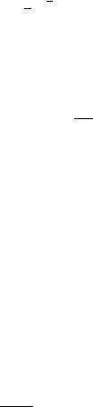
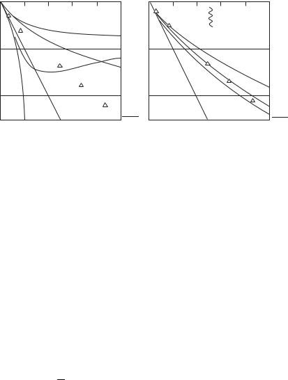
Fig. 5.5. Internal energy of the OCP, as given by di erent asymptotic approximations before

(a) and after (b) the correction, in accordance with relations (5.25)–(5.27) (Gryaznov and Iosilevskii 1973).

In this approximation,

Figures 5.5 and 5.6 show the results of four approximations before and after the correction, which is analogous to that described above: Linearized and nonlinearized Debye approximations (LDH and DH), the Debye approximation in a grand canonical ensemble (GDH), and approximations which asymptotically take into account the dependence of the screening distance on Γ (MN) (Mitchell and Ninham 1968; Guttman et al. 1968; Cohen and Murphy 1969). One can see that this correction improves considerably the agreement with computer experiment (MC), even in the cases when the oscillations of the correlation functions occur in the numerical solutions (Hirt 1967; Hansen 1973; Carley 1974) (behind the wavy line in Fig. 5.5).

Gryaznov and Iosilevskii (1976) have constructed a model describing the oscillations of g(x) (LDH**):

where A and B are the normalization constants, R = R(A, B). The MSA theory (Lebowitz and Percus 1966), as well as the MN model, satisfies the criteria (5.25)–(5.28) and at the same time, as shown by Gillan (1974), describes well the results of the Monte Carlo calculations (see Fig. 5.6).

Therefore, the satisfaction of conditions (5.25)–(5.28) is an e ective way to check the validity of the results of thermodynamic calculations obtained both