Table 10.2 CGT Comparative Site Type Results67

67Combined locations for Chase include body dump and vehicle drop sites; for Collins, encounter, murder, and body dump sites; and for Wuornos, body dump and vehicle drop sites.

10.3.3 Validity, Reliability, and Utility

10.3.3.1 Validity

For geographic profiling to distinguish itself from geomancy, it should meet certain standards. Scientific methodologies must fulfil three important criteria — validity, reliability, and utility (see Oldfield, 1995). Specification of a methodology’s limitations is also important (Poythress et al., 1993). The CGT model works on the assumption that a relationship, modeled on some form of distance-decay function, exists between crime location and offender residence. The process can be thought of as a mathematical method for assigning a series of scores to the various points on the map representing a criminal’s hunting area. For the CGT model to be valid, the score it assigns to the point containing the offender’s residence (referred to as the “hit score”) should be relatively high; that is, there should be few points within the hunting area with equal or higher scores. This relationship can be shown as a distribution curve indicating the number of points with various scores (see Figure 10.4, derived from the CGT analysis of the Olson case). A uniform distribution assigns the same score to every point, producing a horizontal line. (If N is the total number of points on a map, then the probability associated with each point is 1/N.)

The success of the CGT model is measured by the hit score percentage — the ratio of the total number of points with scores equal or higher to the hit score, to the total number of points within the hunting area. This is equivalent to the percentage of the total area that must be searched before the offender’s residence is found, assuming an optimal search process (i.e., one that started in the locations with the highest scores and then worked down). The extent of the search area — the territory police have to search in order to find the offender

— is equal to the size of the hunting area multiplied by the hit score percentage. The mean hit score percentage is 50% with a uniform distribution. This means

© 2000 by CRC Press LLC

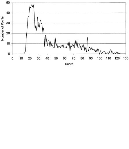
Figure 10.4 CGT score distribution.

that, on average, any police system based on this distribution can expect to locate an offender in half of the hunting area. Investigating suspects alphabetically, tips chronologically, or canvassing from the northwest to the southeast are all examples of such systems.

The validity of the CGT model can be determined by plotting groupings of hit score percentages against those from a uniform distribution (i.e., what is expected by chance) in a Lorenz curve, and then applying an index of dissimilarity or concentration. One such measure is the Gini coefficient (Goodall, 1987; Taylor, 1977). In this case it is equal to:

The Gini coefficient ranges from 0 to 100, with 0 indicating exact correspondence between the two sets of percentage frequencies, and 100 indi-

© 2000 by CRC Press LLC

cating a complete lack of correspondence. The more successful or valid the CGT model, the closer the Gini coefficient is to 100. The distribution of CGT hit score percentages found in the SFU serial murder study was compared to that expected by chance (testing and learning data sets were different). Specific CGT hit score percentages used in calculating the index of dissimilarity are marked in bold in Table 10.1. Degree of offender choice was the basis for determining which score to use when different scenarios were available. This meant that encounter sites were preferred over body dump sites, unless the former were unknown or the target backcloth was patchy (e.g., a red-light district). Also, the dominant residence was used in cases involving more than one offender. Based on 5% intervals, the Gini coefficient for the study sample equals 85, indicating a high level of validity.

An alternative measure of performance can be obtained by doubling the mean hit score percentage; the lower this value the greater the predictive power of the model. This measure ranges from 0, indicating optimal performance, to 1, the value expected by chance. The mean hit score percentage for the above cases is 6.0%, therefore this measure is equal to approximately 0.12. All else being equal, this suggests an area search conducted through a geoprofile would find, on average, the offender’s residence in 12% of the time that a random search would take. The relative performance of the CGT model is therefore approximately 830% (100/12).

Results of the SFU serial murder study show a mean CGT hit score percentage of 6.0% and a median of 4.2% (standard deviation = 4.8); the average number of crime locations was 11.6 (see Table 10.1). Performance ranged from a low of 1.1% to a high of 17.8%. A review of solved operational cases by the Vancouver Police Department Geographic Profiling Section found similar results, with a mean CGT hit score percentage of 5.5% and a median of 4.8% (standard deviation = 4.6); the average number of crime locations was 19.1. Performance ranged from a low of 0.2% to a high of 17.2%. Figure 10.5 shows the distribution of CGT hit score percentages for the SFU serial murder data and a sample of VPD operational cases.

The theoretical maximum efficiency of the CGT model was estimated through Monte Carlo testing, using a computer program to generate random crime site coordinates based on a fixed-buffered distance-decay function.65 The testing produced the “learning curve” in Figure 10.6, which displays the relationship between number of crime sites and median hit score percentage (standard deviation is also shown). Because the distribution is not normal (see Figure 10.5) the median is a better indicator of typical performance than the mean. Functions based on these curves are used in geographic profiling

65 This function produces a pattern similar to Rengert’s (1996) bull’s-eye distribution. The CGT model showed a small drop in performance when tested on other forms of crime site geography (teardrop, bimodal, or uniform spatial patterns).

© 2000 by CRC Press LLC

Figure 10.5 CGT operational performance.

Figure 10.6 CGT model learning curve.

© 2000 by CRC Press LLC