Diss / (Springer Series in Information Sciences 25) S. Haykin, J. Litva, T. J. Shepherd (auth.), Professor Simon Haykin, Dr. John Litva, Dr. Terence J. Shepherd (eds.)-Radar Array Processing-Springer-Verlag

292 T.V. Ho and J. Litva

Dr. Bill Gabriel for carefully reading the chapter and for his comments on the completeness of the material contained herein. As well, we wish to thank Dr. Terry Shepherd for providing a critical and valuable review of the chapter. Finally, we wish to thank a close colleague, Dr. S. Haykin, for helpful suggestions and comments.

References

6.1R.A. Monzingo, T.W. Miller: Introduction to Adaptive Arrays (Wiley, New York 1980)

6.2S. Haykin (ed.): Array Signal Processing (Prentice-Hall, Englewood Cliffs, NJ 1985)

6.3c.R. Ward, A.J. Robson, P.J. Hargrave, J.G. McWhirter: Application of systolic arrays to adaptive beamforming, lEE Proc. Vol, 131, Pt. F, 638--645 (1984)

6.4c.R. Ward, P.J. Hargrave, J.G. McWhirter: A novel algorithm and architecture for adaptive digital beamforming. IEEE Trans. AP-34, 338-346 (1986)

6.5J.V. McCanny, J.G. McWhirter: Some systolic array developments in United Kingdom. IEEE

6.6D.M. Boroson: Sample size considerations for adaptive arrays. IEEE Trans. AES-16, 842-845 (1980)

6.7W.F. Gabriel: Spectral analysis and adaptive array superresolution techniques. Proc. IEEE 68, 654-666 (1980)

6.8R.T. Compton, Jr.: Improved feedback loop for adaptive arrays. IEEE Trans. AES-16, 159-168 (1980)

6.9D.J. Chapman: Partial adaptivity for large array. IEEE Trans. AP-24, 685-695 (1976)

6.10E. Brookner, J.M. Howell: Adaptive-adaptive array processing. Proc. IEEE, 74, 602-607 (1986)

6.11V.U. Reddy, A. Pauiraj, T. Kailath: Performance analysis of the optimum beamformer in the presence ofcorrelated sources and its behaviour under spatial smoothing. IEEE Trans. ASSP- 35,927-936(1987)

6.12T.J. Shan, T. Kailath: Adaptive beamforming for coherent signals and interferences. IEEE Trans. ASSP-33, 527-536 (1985)

6.13W.F. Gabriel: Using spectral estimation techniques in adaptive processing antenna systems. NRL Report 8920 (October 1985)

6.14A.P. Howells: Intermediate frequency side-lobe canceller. U.S. Patent 3202990 (Aug. 24, 1965)

6.15S.P. Applebaum: Adaptive arrays. Syracuse Univ. Res. Corp., SPL TR 66-1, (Aug. 1966)

6.16B. Widrow, P.E. Mantey, L.J. Griffiths, B.B. Goode: Adaptive antennas systems, Proc. IEEE 55,2143-2159 (1967)

6.17L.J. Griffiths: A simple adaptive algorithm for real-time processing in antennas arrays. Proc. IEEE 57,1696-1704 (1969)

6.18O.L. Frost III: An algorithm for linearly constrained adaptive signal processing. Proc. IEEE 60, 926-935 (1972)

6.19M. Klemes: A practical method for obtaining constant convergence rates in LMs adaptive arrays. Trans. IEEE AP-34, 440-446 (1986)

6.20I.S. Reed, J.D. Mallett, L.E. Brennan: Rapid convergence rate in adaptive arrays. IEEE Trans. AES-IO, 853-863 (1974)

6.21J. Capon: Probability distributions for estimators of the frequency wavenumber spectrum. Proc. IEEE 58, 1785-1786 (1970)

6.22J.E. Hudson: Adaptive Array Principles (Peregrinus, Stevenage, UK 1981)

6.23B. Widrow, S.D. Steams: Adaptive Signal Processing (Prentice-Hall, Englewood Cliffs, NJ 1985)

6.24R.T. Compton, Jr.: Adaptive Antennas: Concepts and Performance (Prentice-Hall, Englewood Cliffs, NJ 1988)

6.25S. Haykin: Adaptive Filter Theory (Prentice-Hall, Englewood Cliffs, NJ 1986)

6.26Special Issue on Adaptive Arrays. IEEE Trans. AP-24, (Sept. 1976)

6.27Special Issue on Adaptive Processing Antenna Systems. IEEE Trans. AP-34, (March 1986)

6.28W.F. Gabriel: Adaptive arrays-an introduction. Proc. IEEE 64, 239-272 (1976)

6.29H.T. Kung, W.M. Gentleman: Matrix triangularization by systolic arrays, in Real-Time Signal Processing IV, Proc. SPIE 298, 19-26 (1981)

6.30J.G. McWhirter: Recursive least-squares minimization using a systolic array, in Real-TJme Signal Processing VI, Proc. SPIE 431, 105-112 (1983)

6.31R.T. Compton: An adaptive array in a spread-spectrum communication system. Proc. IEEE 66, 289-298 (1978)

6.32J.H. Winters: Spread spectrum in a four-phase communication system employing adaptive antennas. IEEE Trans. COM-30, 929-936 (1982)

6.33H. Steyskal, J.F. Rose: Digital beamforming for radar systems. Microwave 32, 121-136 (1989)

6.34G.H. Golub: Numerical methods for solving linear least-squares problems. Numer. Math. 7, 206-216 (1965)

6.35W. Givens: Computation ofplane unitary rotations transforming a general matrix to triangular form. J. SIAM 6, 26-50 (1958)

6.36W.M. Gentleman: Least-squares computations by Givens transformations without squareroots. J. Inst. Math. Appl. 12,329-336 (1973)

6.37T.V. Ho, J. Litva: Systolic array for 2D adaptive beamforming, IEEE Int'I Conf. on Systolic Arrays, San Diego, CA, May (1988)

6.38M.M. Hadhoud, D.W. Thomas: The two-dimensional adaptive LMS algorithm. IEEE Trans. CAS-35, 485-494 (1988)

6.39S.T. Alexander, S.A. Rajala: Image compression results using the LMS adaptive algorithm. IEEE Trans. ASSP-33, 712-714 (1985)

6.40Y.L. Hong, C.c. Yeh, D.R. Ucci: The effect of a finite-distance signal source on a far field steering Applebaum array-two-dimensional array case. IEEE Trans. AP-36, 468-475 (1988)

6.41M.P. Ekstrom: Realizable Wiener filtering in two-dimensions. IEEE Trans. ASSP-30, 31-40 (1982)

296 B.D. Steinberg

different for mechanically-induced phase errors resulting from geometric distortion. For this situation signals must arrive at the distorted array from outside the system; these signals must be measured by the system after all the distortioninducing sources have operated, and a wavefront or phase aberration correction deduced from the measurements.

This procedure is called adaptive beamforming, to which the acronym ABF is given in this chapter.

The remaining difficult problems are matters of practicality. A two-dimen- sional optical aperture 105 wavelengths in diameter is a relatively simple device. The corresponding microwave phased array is a horror, however. Its area is the order of 1010 square wavelengths, with elements spaced A./2 to ensure the avoidance of grating lobes. The number of antennas, phase-shifters for beam steering, and receivers are about 4 x 1010• Drastic thinning by several orders of magnitude is required to constrain cost. Thinning can be periodic, provided that procedures are introduced that avoid the problems of grating lobes, or aperiodic.

A second practical problem is the cost and complexity of the intra-array communications subsystem. Its function is to transfer the signals received at the array elements to the signal processor. The number of communication channels equals the number of antenna elements. Call this number N. Each channel is sampled at the rate B, which is the order of the signal bandwidth. Each sample is quantized into b bits. The product N Bb is the data transmission rate. It is easily shown that this number can be excessively large. Consider a one-dimensional linear array of 105 wavelengths designed to provide a resolution cell of 1 meter in both range and cross range. The number of antenna elements in a filled array is N = 2L/A., and the signal bandwidth is 150 MHz. Each I/Q component of the coherently demodulated signal will be quantized to 6-8 bits. Therefore, b = 12-16. The product NBb exceeds 1014 bps, which is larger by several orders of magnitude than the transmitter frequency, and is hopelessly beyond our technological capability. N is reduced by thinning; b can also be reduced to some extent.

7.2 Adaptive Beamforming: Dominant Scatterer Algorithm

Figure 7.1 shows a badly distorted receiving antenna array in the upper-left portion. Each receiving element drives a coherent receiver, whose outputs are sampled and stored. The transmitter, also shown in the upper-left, radiates a short pulse toward the target area to be imaged. A prominent scatterer, modeled as a corner reflector in the figure, is in the general direction of the target region. The illuminating beam is broad in azimuth, as is common in radar; the beamwidth is typically a few degrees. This beamwidth defines the instantaneous field of view of the imaging system. That is, the system can only image those targets that are illuminated by the transmitter. A typical received waveform is

7.3 Experiments

This algorithm has been used repeatedly at the Valley Forge Research Center of the University of Pennsylvania over the last decade and a half. It is a very robust procedure. The echo from the dominant scatterer need only be 4 dB larger than the sum of all the echoes from the clutter. Figure 7.2 shows a high-resolution image of a street of row houses in a town about 6 km from the laboratory [7.4J. The phased array was highly distorted; the distortion was estimated to be about one wavelength rms in all dimensions. The diffraction-limited image obtained with the dominant scatterer algorithm exhibits cross range resolution of 3 m,

6490-

~-

6350-

Cross-range (meters)

(a)

Fig, 7.2. Images of row houses on two streets of Phoenixville, PA, at a distance of 6.5 kIn from the Valley Forge Research Center, comparing (a) adaptive and (b) nonadaptive beamforming. A= 3 cm, ~R (range cell) = 3m, ~S (cross range cell) =:< 2.5 m. [7.10]

300 B.D. Steinberg

consistent with the antenna size (83 m), wavelength (3 em) and target range. The range resolution was 3 m, determined by the duration of the 20 ns pulse. The lower portion of the figure shows the image from the same data set without adaptive beamforming. It is a useless jumble of pixels. Adaptive beamforming converted a hopeless condition into a useful imaging procedure. Figure 7.3

Azimuth (milliradians)

(b)

I

I

I

I

I

I

I

IL.. ___ _

Fig, 7.3a, b. Diffraction-limited 3 em radar map of suburban housing development, Phoenixville, PA, showing streets and houses. Each pixel cluster is a house. The houses are about 20 m apart. Resolution is comparable to human vision. (b) Plan of the housing development. [7.10]

shows a suburban housing development 4.5 km from the laboratory. Each clump of pixels is a single house. The houses are spaced by approximately 20 m. Streets and backyards are evident. The cross range resolution in Figs. 7.2 and 3 is comparable to human vision.

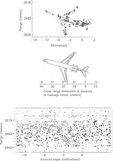
The same algorithm can be applied to a succession of pulse echoes received from a moving target by a monostatic radar. The technique is called inverse synthetic aperture radar (ISAR). The line of sight direction to the target changes from pulse to pulse due to the target motion (Fig. 7.4, left). From a frame of reference on the target (right), the apparent location of the radar moves from pulse to pulse. This sequence of apparent locations forms a synthetic aperture. The pulse sequence received by the radar is treated as if each pulse train came from a different antenna element. The data are laid down in a store exactly as in Fig. 7.1, and are processed as in Tablet.l. An example of the result is shown in Fig. 7.5, which is a high-resolution two-dimensional image of a Boeing 727 flying into Philadelphia International Airport. This ISAR image was obtained with adaptive beamforming. The bottom of the figure is the image of the same data when adaptive beamforming was not included. Again, the comparison is striking.

The two techniques can be performed simultaneously to provide a combined spatial-temporal radio camera. Figure 7.6 shows the result of such an experiment. The receiver was a two-element interferometer in which the elements were spaced at 25 m. Eighty-five echo traces were obtained from each receiver from a

5

Fig. 7.4. It is also possible to apply radio camera processing to a sequence of echoes from a moving target, received by a single antenna. An inverse synthetic aperture is formed. Adaptive beamforming corrects for distortion in the synthetic aperture caused by flight-path deviations. Image processing is the same as in the spatial radio camera. (From [7.5])