Diss / (Springer Series in Information Sciences 25) S. Haykin, J. Litva, T. J. Shepherd (auth.), Professor Simon Haykin, Dr. John Litva, Dr. Terence J. Shepherd (eds.)-Radar Array Processing-Springer-Verlag
.pdf80 U. Nickel
the expensive maximum likelihood estimations (calculation ofthe denominator). In addition, if all tests use different data vectors and are therefore, independent, the probability for deciding for HM is the product of the probabilities for the decision at each stage, i.e.,
P(HM) = P[2ln(Td> 111] .. .. P[2In(TM-d>'7M-l}P[2ln(TM)<'7M]·
This means that, asymptotically, the probability to overestimate the number of targets is bounded by the chosen error level of the test HM , because we can choose '7M such that, asymptotically,for all M P[2ln(TM) < '7M] = 1 - 0(. This sequence oftests with respect to M is a sequential multi-hypotheses test with fixed asymptotic error level (over-estimating the target number).
White Noise Tests [3.59]. When w~ use a suboptimum parameter estimation procedure, e.g., stochastic approximation, we may construct a similar sequence of tests with the same asymptotic properties as the likelihood ratio test described previously. Instead of the likelihood ratio, we use as a test statistic the function Q(wmin ) (3.28-31), where Wmin has been found by some suboptimum minimization procedure. Assuming that the sUboptimum minimization is consistent, 2Q(Wmin) is asymptotically X2-distributed with K (2N - 2M) degrees offreedom. Thus, we have a sequence of tests with the same properties as before.
Information-Theoretic Criteria [3.61]. The information-theoretic criteria AIC [3.20, p. 234], MDL [3.26] mentioned in Sects. 3.2.3, 3.2.5a and in Chap. 2, can also be applied to this problem. The corresponding expressions for these criteria are given in Chap. 2 (2.54,55). Simulations showing the required signal-to-noise ratios for some scenarios have been published in [3.61]. In these simulations, the MDL criterion proved to be the best among the information theoretic criteria. The disadvantage of these procedures is that the time consuming parameter estimation has to be done for all hypothetical target numbers. This is prohibitive for real time applications.
d) Experimental Results
The key proof of the usefulness of superresolution methods is to conduct experiments with real data. A number of different experiments have been conducted which support the impression that PTMF methods are best suited for the special radar angular resolution problems listed in Sect. 3.1.1.
Most ofthe results presented in the open literature are for low angle tracking data. In [3.72], resolution ofmultipath components with the double-null tracker of White is reported: For two paths separated by half a beamwidth a tracking accuracy of more than 0.1 beamwidth was achieved. This is the accuracy of the raw double-null tracker angle estimates averaged in some way. A very stable (strongly coherent) multipath situation was analyzed in [3.73]. Again, separations down to about 0.5 beamwidth were resolved. The errors depended strongly on the phase difference between the direct and reflected paths. These experiments were done without a target number determination.
3. Radar Target Parameter Estimation with Array Antennas |
81 |
Our experience with real data indicates that the resolution of targets at 0.5 beamwidth is, in general, possible with PTMF methods, even with some system errors. However, resolution below this value is difficult to achieve, and the required system accuracy increases non-linearly with the resolution gained in fractions of the beamwidth. This is the typical behaviour for methods based on the standard signal model in (3.24). For the refined multipath model used in [3.8], we have a completely different parameterization, and the behaviour is different.
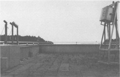
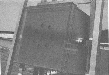
Experience with real data has been gained at FGAN-FFM with a small system designed for superresolution called DESAS (DEmonstration of Superresolution Array Signal processing). DESAS consists of a small planar receiving array and three dipole antennas for simulating targets. The arrangement is shown in Fig. 3.10. The target antennas can be fed with the same, or different (uncorrelated) CW sources, or with white noise. One antenna can be moved to produce target separations from 1.5 to 0 beamwidth. Figure 3.11 shows the 8- element planar receiving array. The positions of the elements are irregular. The receiving array works at S-band. All element outputs are digitized with 9 bits and processed by a microprocessor. This not only allows for examination of different algorithms, but also of the influence of software calibration procedures (Sect. 3.2.7).
The PTMF method by stochastic approximation (Sect. 3.2.6b) together with the white noise test (Sect. 3.2.6c) is implemented. This combination has been extended to a fully adaptive method by also allowing a reduction of the target number. Too large a target number is detected by examining the estimated power of each target. If the averaged target power is too low, this direction is
Fig. 3.10. FFM-DESAS experimental set-up: receiving array and 3 sources for simulating targets
82 U. Nickel
Fig. 3.11. FFM-DESAS experimental set-up: 8-element irregular receiving array
neglected and the target number is reduced. As the PTMF method always has difficulties in correctly identifying closely spaced targets, a third criterion is introduced for practical reasons: If the target directions are too close together (closer than we expect to be resolvable for the given algorithm), then these two directions are considered as one target and the target number is reduced. Figure 3.12 shows a block diagram of the complete adaptive closed-loop superresolution algorithm. The order of the tests is not arbitrary; it affects the stability of the procedure.
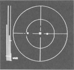
Figure 3.13 shows the output display for a three-target estimation problem. The 3 dots within the circles show the directions of three targets estimated by
direction estimation by stochastic approximation
|
Fig. 3.12. FFM-DESAS: Structure |
r--:--~---,yes |
of closed-loop adaptive superresol- |
t-------tM = M + 1 |
ution with angle estimation and |
|
target number determination |
3. Radar Target Parameter Estimation with Array Antennas |
83 |
Fig. 3.13. FFM-DESAS display of results from closed-loop superresolution by stochastic approximation and multi-hypotheses test
stochastic approximation. The size of the dots is proportional to the estimated actual amplitude of the individual targets. In this example, the directions correspond to the true directions with an accuracy better than 0.1 beamwidth. The inner circle indicates the size of the 3 dB beamwidth of the antenna, and this gives an impression of the separation between the sources. Target separations are approximately 0.5 BW and 0.3 BW. The bars on the left side represent the test statistics. The 3 bars farthest to the left indicate the test statistic for reducing the target number. The test criterion for this is the estimated target power, averaged over a sliding window of suitable length. The crossline indicates the threshold. The vertical bar farthest to the right shows the test statistic for increasing the number of targets according to the white-noise test described before. We may switch the different sources on and off or move the antennas, and the system displays the target parameters in real time. This is the degree of automation we need for future phased array radar. With this arrangement, we are able to demonstrate superresolution of targets down to 1/5 of a beamwidth, if the target number is known. If, however, the target number is unknown, the separation has to be slightly greater. This is because the closed-loop adaptation procedure is slower for small target separations, in which the procedure does not follow a blinking target situation.
3.2.7 Aspects of Implementation
An important problem to be considered is how the array outputs, which are necessary for superresolution, are generated. We may have special arrays dedicated to one of the tasks listed in Sect. 3.1.1, or a large multifunction phased array radar.
84 U. Nickel
a) Superresoiution Arrays
If high resolution in both azimuth and elevation is required, then we must have a planar array. For a typical multi-function phased array radar with thousands of elements, it is presently too expensive to digitize all element outputs. Therefore, subarrays are used to reduce the number of channels. The choice of the subarrays is an important design issue for a multi-function phased array radar because this is a decision involving many different radar problems: antenna sidelobe reduction, difference beamforming, adaptive jammer suppression, and superresolution.
The positions of the centres of the subarrays constitute a "superarray". If we apply superresolution methods to the subarray outputs, we may consider this as using the superarray with array elements having a pattern corresponding to the subarray pattern. The superarray essentially determines the resolution properties. To produce the best resolution, this superarray should cover the whole aperture, i.e., all elements should be used. We can show that if we have a regular fully filled array (which will be chosen if a low sidelobe antenna is desired), we should then avoid regular subarrays because of the grating lobe problem [3.74]. Grating lobes [3.74] arise because the superarray positions have distances greater than the half wavelength. This results not only in a periodic repetition of the high resolution angular spectrum, but also in a folding-in of targets outside the angular regions of interest. If we choose subarrays of a different shape, such that the array of the subarray centres (the superarray) is randomly distributed, we can avoid grating lobes. However, for the signal model inherent in the superresolution methods, an equal array element antenna pattern is required. Experiments show that if the number of subarrays is sufficiently high (more than twenty), and if we are not interested in extremely high resolution, we need not correct for the different subarray patterns because the errors tend to average out [3.75]. Of course, if we want to attain the ultimate limit in superresolution, we then have to correct for the subarray patterns.
For the special application of low angle tracking we need only one-dimen- sional (elevation) resolution. More simple superresolution arrays are possible in this case. One may extend a conventional reflector antenna by adding a column of, say, 10 antenna elements, with all element outputs converted to digital form. If we have a planar array, we can take rows of elements as subarrays to generate a vertical superarray with digital element outputs. Many of the current rotating and vertically electronically scanning radars are of this type. The subarrays are, in this case, all equal and at AI2 spacing such that the methods can be applied without any corrections. Of course, a fully 2D-electronically scanned array with random subarrays is also well suited; rows of subarrays could then be in conflict with other tasks (e.g., adaptive nulling).
To reduce the processing complexity we would like to use as few channels (subarrays) as possible. This raises the question as to what the minimum possible number of channels should be. To resolve M targets, we need a certain number N of array channels such that the assumed signal model can be
3. Radar Target Parameter Estimation with Array Antennas |
85 |
identified, i.e., the parameters can be uniquely determined. This is not simply a matter of counting the number of unknowns and data samples, because we have a nonlinear estimation problem to deal with. For arbitrary arrays it is difficult to determine the minimum number N. For a linear array at )../2 spacing we may show that N - 1 uncorrelated targets can be resolved, and N/2fully correlated targets, e.g., fixed phase relations, can be resolved, (see [3.76] and references cited therein). For a planar array with N elements on a rectangular grid, we may
require these regularity conditions for the rows and columns; that is M = .j"ii=t and M = .JN7i are the maximum number of resolvable targets
for uncorrelated and correlated targets, respectively. For irregularly spaced arrays (subarray centres), the maximum number of resolvable targets is generally higher.
In order to reduce the computational complexity, we would like to use the minimum number of channels. However, we then have to require the highest accuracy for these channels. In most cases, the channel accuracy requirements are tougher to satisfy than the amount of computations. The use of a number of channels as large as possible represents a more robust solution.
b) Array Accuracy
If modern superresolution algorithms are to perform as powerfully as they do in simulation, extremely accurate measurements are required. It is not reasonable to simply ask for hardware with high precision, because this would raise the cost of building the system to an unacceptable level. Most errors can be compensated for by software. This is done by inserting special test signals at suitable points in the receiving chain. Antennas with this property are called self-calibrating antennas. This is a key technique in practical implementation of modem array signal processing algorithms.
The first problem is the accuracy of each single channel. Typical errors arise from mixing down to baseband: different offset and amplification for the I and Q channels, and orthogonality errors between the two channels. If we insert a suitable signal at IF, we can measure these errors and can transform the I and Q channels into error-free channels, provided the dynamic range of each channel (number of bits used in the AID converters) is sufficient.
The second problem is the equality of all channels. Between the different array channels we have phase and amplitude errors resulting from different element patterns (which may be the subarray patterns), different cable lengths, amplifiers, etc. We may use an external source in the far field or near field of the antenna, or insert a test signal directly behind the antenna elements to measure these differences, and then multiply each channel with the inverse complex value. There are many practical problems associated with the different methods of inserting a calibration signal. The important point to note is that with self-calibrating antennas we only require that the channels be stable in time.
86 U. Nickel
Channel accuracy requireinents also decrease with an increasing number of channels, provided the beamwidth remains the same. For robustness we, therefore, prefer to have as many subarrays as the financial budget allows.
3.3 Frequency Estimation
Frequency estimation is mathematically equivalent to angle estimation, because in both cases, we perform a finite version of the discrete Fourier transform, the so-called periodogram. The spatial sampling points Xi convert into time sample points t", the direction sine u converts into the angular frequency Q) = 21tf
However, the type of data used is different: we do not have different realizations (snapshots) of the random data vector, but one realization of the underlying stochastic process. Normally we have equally spaced time samples (exception: staggered pulses), and for a phased array radar the time series can be made nearly as long as desired. The length of the time series, and that means the spectral resolution, is only limited by the time for which the target is within the angle-range-doppler resolution cell. For highly manoeuvring targets this can be about 1-2 seconds, which corresponds to some 1000 pulses, i.e. time samples.
3.3.1 Doppler Filter Bank
The usual method to determine the frequency shift of radar target echoes is to use a Doppler filter bank. The main purpose of the Doppler filter bank is to perform coherent integration and clutter suppression. The Doppler filter bank is a hardware realization of the discrete Fourier transform (DFT), or the fast Fourier transform (FFT). The maximum number of pulses is hardware-limited, e.g. to 32, 64, etc. The channel with maximum output power is taken for the corresponding frequency. For a more accurate single target frequency estimation we may interpolate the output values of adjacent channels, because the single channel Doppler filter characteristic is known. These techniques are analogous to the angle estimation problem with array antennas, and work ifit is known that there is only one target present. The resolution of multiple targets is not enhanced by Doppler channel interpolation. The (conventional) resolution is limited by the 3 dB width of the filter channel passband. This is, therefore, the normal separation of the centre frequency of the different filters.
Low Sidelobe Doppler Filter. A common radar problem is detecting targets in the presence of strong clutter. In this case, the first sidelobe of the Doppler filter, which is at - 13 dB, may be too high to suppress the clutter. Therefore, weightings or window functions for reducing the principal filter sidelobes are often applied. This is analogous to the reduction of antenna sidelobes by tapering. Different taper or window functions, e.g., Hanning, Hamming, Parzen [3.20, 23], are used. A common property of these weightings is that by reducing
3. Radar Target Parameter Estimation with Array Antennas |
87 |
the sidelobe level, the filter mainlobe is made broader and resolution is reduced. So, these techniques for clutter suppression have detrimental effects on the estimation of the target echo frequency. This degraded estimation accuracy is often accepted for the enhanced clutter suppression that is gained. Good estimates of the target velocity are also provided by modem target tracking algorithms (e.g., the Kalman filter).
3.3.2 Superresolution Methods
Applications. Interest in high-resolution frequency estimation methods for use in radar arises from applications that involve target classification. We may try to distinguish between jet or propeller driven aircraft, helicopters, or even to identify the exact type of an aircraft. One way to achieve this is by analyzing the echo spectrum which may exhibit typical spectral lines from the echoes of the rotor blades. Another way is to increase the angular resolution by SAR (Synthetic Aperture Radar) or ISAR (Inverse Synthetic Aperture Radar) techniques. SAR exploits the fact that the time samples of a radar on a moving platform can also be interpreted as spatial samples of a (possibly) large aperture along the path of the radar within the observation time. This can give extremely high angular resolution provided the path geometry is known exactly, and the target is fixed within the observation time. The radar platforms can be very different: an aircraft (for reconnaissance), a satellite, or the rotating earth itself (in radio astronomy). If a ground-based radar tracks a moving target we have a similar situation. If we change our coordinate system into that of the moving target, the radar apparently is moving around the target, and we may again apply SAR processing; such a method is called ISAR. ISAR can resolve an aircraft into single scatterers, provided the target movement - and this means not only the path, but also all parameters of the attitude, pitch, roll, and yaw - is known exactly. The main problems of SAR and ISAR processing are path corrections and auto-focusing techniques for the synthetic array. When the data have been transformed according to the synthetic aperture, again, a spectral analysis is performed and superresolution methods may be applied.
The resolution with SARjISAR is mainly determined by the accuracy of the array focusing technique and much less by the spectral estimation method used. The focusing accuracy determines how large the synthetic aperture can be made. When the aperture has been extended as much as possible for the robust use of the periodogram, we cannot expect to gain anything with the use of sensitive superresolution methods. Classification by target echo spectral analysis, SAR, and ISAR are the main applications of superresolution methods for radar frequency estimation.
A typical feature of target classification is that in many cases we are not directly interested in the spectrum; rather, we derive from the time series a set of target description parameters, which is then compared with a target library for classification. This set of parameters may be the frequencies of typical spectral lines, the AR coefficients of the estimated spectrum, or a set of orthogonal
88 U. Nickel
vectors representing the signal subspace. We only need convenient data reduction for the complex target characteristic. In this case, we also do not have the detection problem of extracting some of the largest peaks of the estimated spectrum, as mentioned in Sect. 3.2. Instead, we have the problem of allocating a target in our library to the set of parameters found (e.g. by finding the nearest neighbour with respect to a suitable metric). If we use a PTMF method, we may simply take the parameter sets from the target library and check which particular one fits the measured data best (no minimization of the function (3.26) is necessary). These problems are different from the typical parameter estimation and resolution problems; they will not be considered here. However, this indicates that the intensive research on superresolution spectral analysis which focuses only on sharp spectral peaks is not of interest for some real radar applications.
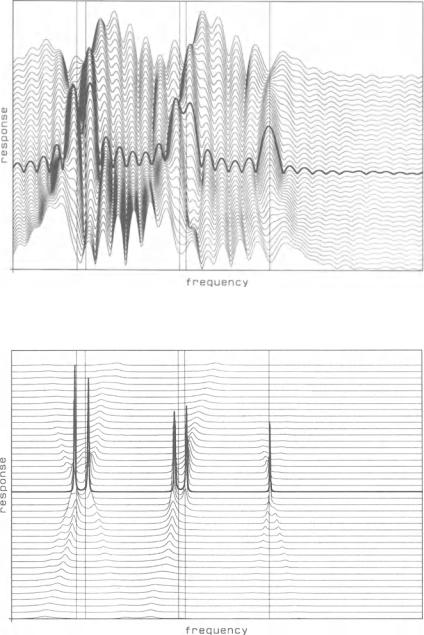
Choice of Method. All the methods discussed in Sect. 3.2 are applicable to frequency estimation. The spectral estimation methods which are restricted to linear, equally spaced arrays, like the ME, AR and Kumaresan-Tufts methods, are of particular interest if we want to know the shape of the spectrum without extracting spectral lines (e.g. for visual inspection). There is sufficient material available on spectral estimation with these methods [3.22, 23J, to which the interested reader is referred. The decision as to which method is best suited, has to be made for each individual application, taking into account the type ofsignal one is interested in, and the type of errors present. We will illustrate this by a simulation with SAR data.
The SAR data have to be corrected with a phase contribution according to the motion of the platform. Linear phase compensation is the normal motion compensation technique. SAR data are, therefore, typically corrupted by quadratic phase errors. Figures 3.14-16 show typical spectra with quadratic phase errors. Four spectral lines at 20 dB signal-to-noise ratio are present, grouped in two pairs separated at 0.5 and 0.7 beamwidth. A fifth, isolated, spectral line is at 14 dB SNR. The frequencies of the spectral lines are indicated by vertical lines. The length of the data sequence is 64. We have plotted the time history of the estimated spectra (waterfall plot). Motion compensation has been done at time tc in the middle of the plot (spectrum with bold line). Before tc we have negative quadratic phase errors, and afterwards, positive errors. The maximum phase error (top and bottom spectrum) corresponds to 2n from the beginning to the end of the time series. Figure 3.14 shows that the conventional fast Fourier transform (FFn algorithm is not useful, even with correct focusing, because the line pattern is masked by the sidelobes. The Burg algorithm in Fig. 3.15 (modelorder set equal to 20) estimates the pattern oflines with some bias that increases as the phase errors increase. This could lead to a wrong classification of the target at tiines too far away from tc' The MUSIC algorithm (with spatial averaging down to dimension 20, with the dimension of signal subspace set equal to 5) in Fig. 3.16 only exhibits spectral lines for correct motion-compen- sated data and nothing for erroneous data. It is, in fact, a matched filter for the