Diss / (Springer Series in Information Sciences 25) S. Haykin, J. Litva, T. J. Shepherd (auth.), Professor Simon Haykin, Dr. John Litva, Dr. Terence J. Shepherd (eds.)-Radar Array Processing-Springer-Verlag

62U. Nickel

3)The spatial samples may not be equally spaced. For large planar antennas, we have to work with subarray outputs as spatial samples. The subarray centres should not be on a regular grid.

4)There are problems with two-dimensional generalization ofthe linear prediction approach. For two-dimensional irregular arrays, the method of linear prediction is not applicable.

3.2.4 Capon-Pisarenko-Type Methods

These methods use spectral estimates of the form

where Ris some covariance matrix estimate, as in Sect. 3.2.2, and r is a positive and real constant. The case of r = 1is due to Capon, [3.20, p. 119J; the extension to an arbitrary r was presented by Pisarenko [3.31J; for r = 2 this is also called a "thermal noise algorithm" which has attracted some attention [3.32]. In this category we also summarize methods which use combinations for different r, like the "adaptive angular response" method [3.33J, which is the ratio Sc.2(U, V)2/Sc.l (u, v), or the "Rayleigh estimate" which is Sc.r+ 1(u, V)r+ 1/Sc.r(U, v)' [3.34].

All these methods are applicable to random planar arrays. However, they apply to fully correlated targets only if spatial smoothing is possible. The methods have a good detection performance; that is to say, the distribution of the estimated spectrum is not very heavy tailed for a sufficiently large number of samples [3.20, p. 162; 31]. A typical feature of these methods is the large amount of computations (matrix inversion, possibly multiplication) and the moderate resolution. The Capon method, which can be considered as the fastest member of this class, has less resolution than the methods of all other classes. The Capon method has the advantage that the value of the peaks of the spectrum gives a good estimate of the source power, but, as mentioned in Sect. 3.1, this is not an important parameter in the case of radar. The Capon-Pisarenko approach is, therefore, not very well suited for radar.

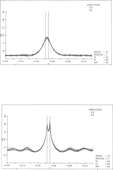
To give an example of the performance of the Capon method, we consider the following standard example (A):

A)A linear antenna with N = 64 elements at A/2-spacing, two uncorrelated Gaussian targets separated by 1/2 BW, input single target signal-to-noise ratio: 9.5 dB, covariance matrix estimated from 43 data vectors (small sample-size performance).

To give a feeling for the fluctuations of the spectra we always plot 10 different realizations.

Figure 3.4 shows the performance of the Capon method for this standard example. The estimated covariance matrix from 43 data vectors is not invertible, therefore, the dimension is reduced by spatial averaging. A reduction to a

64 U. Nickel

shows the corresponding result for the AR method in comparison. The same 33 x 33 spatially averaged covariance matrix was used.

3.2.5 Signal Subspace Methods

For this class ofmethods, it is assumed that the signal vectors from the targets to be resolved lie in a lower dimensional subspace of the whole complex space of array output vectors. In other words, these methods exploit the fact that the covariance matrix can be written as the sum ofthe signal covariance matrix with lower rank and the noise covariance, which is proportional to the identity matrix. These methods assume a structure of the covariance matrix as in (3.13), but without any specific form of the matrix A except for the dimensions.

If the noise covariance matrix is not proportional to the identity matrix, we need some knowledge about the noise matrix to define a signal subspace. The normal approach is that the noise covariance matrix Q is assumed to be known (or has been estimated), and the array output vectors z are then whitened by multiplying them with a matrix W = Q-l/2 . Q-l/2 denotes any square-root of Q-l, e.g., determined by the Choleski decomposition of Q-l. This technique has been described in the previous chapter for several detection problems; it is the essence of optimum interference suppression. The expected signal is, then, no longer proportional to the vector a(u, v), but to Wa(u, v). For active radar, the noise alone covariance matrix can be estimated from data samples at time instances when no echoes of the transmit signal are to be expected. Prewhitening of the data with a matrix W = Q-l/2 means that the covariance matrix of the whitened array outputs is:

Rw = E{zwz~}

=WE{ZZH} WH

=W(ABAH + Q)WH

The matrix Rw has the same structure as the matrix in (13), which is required for signal subspace methods, but with the matrix Aw = WA instead of A.

Signal subspace methods have attracted a great deal of attention in the past years because of their excellent resolution properties. The main problems with signal subspace methods are how to obtain an estimate of the (orthonormal) basis (Xl'. : . , XM) of the signal subspace, and how to determine a suitable dimension M. For radar applications this decision procedure should be completely automatic. When the signal subspace basis (Xl' ..• ' xM) has been determined, there are two approaches to obtain angle estimates: to calculate an angular spectrum from (Xl' . .. ,XM), or to determine the directions algebraically.

a) Projection Methods

The subgroup of projection methods creates an estimate of the angular power spectral density defined by

where P is a projection matrix. The form of this spectrum is very similar to the Capon spectrum (3.16), for r = 1. P projects on the space orthogonal to the signal space (complement of the signal space, sometimes also called "noise space", although the noise has values in the whole N-dimensional space). If we have an orthonormal basis for the signal space (Xl' .•• ,XM) = X, then P can be represented as:

There are different approaches for getting an estimate of the signal subspace X:

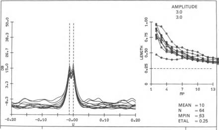
The MUSIC algorithm, (~l)ltiple SIgnal Classification [3.35, 36]). Here X is composed of the dominant eigenvectors ofthe estimated covariance matrix. The covariance matrix may be estimated by the ML method (3.8). Toeplitz structure estimates, spatial smoothing, forward-backward averaging, etc. are also possible. This method is known for its good resolution properties from simulations [3.32] and theory [3.37-39]. With ML estimates for the covariance matrix, the method is applicable to arbitrary arrays. For completely correlated targets, the signal covariance matrix does not have full rank, and the method is not useful, except if we use spatial averaging for a linear, equally spaced array. The degradation for correlated targets has been analyzed by Stoica et al. [3.39], who also give a good review of the properties of the MUSIC method. In particular, it is shown there that for uncorrelated targets, MUSIC performs asymptotically (K -+ (0), the same as the maximum likelihood estimate of (3.25).

Figure 3.6 shows the performance of the MUSIC method for the standard example (A). The performance is much better than the one for the Capon method shown in Fig. 3.4. The dimension of the signal subspace is, in this case, always found to be equal to two, the number of targets. The angle estimate is, in all cases, unbiased up to the plotter grid, which is 0.09 BW.

For many applications the dimension of the signal subspace has to be determined from the data, too. This problem has been treated under different assumptions in the previous chapter under the name 'pseudo ML estimate'; the name refers to the approach that does not estimate the true target parameters, but only a set of vectors spanning the signal subspace. A variety oftests has been presented in the previous chapter. We comment here only on the common approaches to do this.

a) Extended Sphericity Test. This is a sequence of likelihood ratio tests for equality of the N - M lowest eigenvalues of the estimated covariance matrix. No knowledge of the noise power is necessary. This test would, therefore, be

an orthogonal basis of the signal subspace are just the eigenvectors corresponding to the M largest eigenvalues, and the likelihood ratio test for HM results in the test statistic

(3.20)

where the Ai denote the ordered eigenvalues of R, and N denotes the number of array elements. Basically, Twn compares the estimated noise power with the known noise level (12. This test statistic is well approximated by the X2 - distribution with 2K(N - M) degrees of freedom, [3.40]. Simulations have shown that the probability to overestimate the number of targets is, in fact, bounded by the chosen error level of the x2-threshold as is to be expected from theory. The examples shown in Fig. 3.6 were run with this test. The error level was set to 10%. In all ofthe 10 experiments shown in Fig. 3.6 the test has chosen the dimension of the signal subspace to be 2.

c) Information Theoretic Tests. The most popular criteria are the AIC [3.20, p. 234] and the MDL criterion [3.26], that were mentioned previously. For this application, these two criteria estimate the dimension of the signal subspace, M, by respectively minimizing the function

AIC(m) = K(N - m)log[T.ph(m)] + m(2N - m)

and

MDL(m) = K(N - m) 10g[T.Ph(m)] + (1/2)m(2N - m)log(K) .

These criteria have also been calculated in Chap. 2, (2.170, 171). We observe that these criteria are based on different approximations for the distribution of the extended sphericity test statistic. Although the MDL overcomes the inconsistency of the AIC, simulations do not always show superiority of the MDL criterion [3.41, 42]. It has been argued that an advantage of informationtheoretic criteria is that no subjective threshold selection is required. However, correct threshold tests provide a known bound on the probability of overestimating the number of sources. This may be an important figure for further radar data processing to prevent saturation of the system. Information-theoretic criteria have unknown error probabilities.

Tbe Hung-Turner (HT) projection. This method requires less computational expense than the eigendecomposition based approach. The matrix X is estimated by simply orthogonalizing the measured data vectors [3.43, 44]. The motivation for doing this is the fact that if the signal-to-noise ratio is high, the data vectors approximately span the signal subspace.

The orthonormalized columns of the data matrix Z = (Zl, ... , ZK) can be written as

X = Z(ZHZ)-1/2 .

for the first 13 samples is shown in the plot on the right. The average number of samples was 43.1, with minimum and maximum values of 34 and 54, respectively. Obviously, the dimension of the signal subspace of the HT method is no indication ofthe number of targets. The high dimension ofthe signal subspace is necessary to allow some averaging over the dimension. The signal subspace dimensions of Fig. 3.7 are not the numbers with best performance. Smaller numbers ofdata vectors give the same resolution, but a better sidelobe level. The CEL test works well for high SNR (e.g. ifthe HT method is used for interference suppression [3.43,44]), but for typical SNR values for superresolution, it overestimates the optimum dimension of the signal subspace by a factor of 2. It is difficult to find a test procedure that works well for all signal-to-noise ratios.

Although there are some fluctuating sidelobes, this method does not perform badly, considering its simplicity. In aU cases, the sources are resolved. In only one case do we have an angular bias of one plotter grid point, which is 0.09 BW. The problem is that there is only a very limited amount of data averaging possible (in contrast to averaging given by the estimated covariance matrix). The method is applicable to arbitrary arrays, but not for completely correlated targets.

The Yeh-Brandwood (YB) projection. The averaging problem with the HT projection can be overcome if the columns of the estimated covariance matrix are used as a basis for the signal subspace. This idea, mentioned by Hung and Turner [3.43], is investigated in [3.45, 46]. For point targets, the covariance matrix has the form given by (3.13). The columns of the signal-alone covariance matrix obviously span the signal subspace. The problem is to get rid of the noise covariance matrix. Yeh [3.46], uses the columns of the rectangular submatrix below the main diagonal as basis vectors for the signal subspace. This has the effect of neglecting some array element outputs and reducing the given aperture. Simulations and real data experiments with this technique applied to the low angle tracking problem have been presented in [3.10]. Brandwood [3.45], assumes the noise covariance matrix can be measured, and is then subtracted from R. For large, sample size K, these methods should perform the same as the MUSIC method [3.10].

The YB method is applicable to arbitrary arrays, and with spatial averaging, also to completely correlated targets.

The Kumaresan-Tufts (KT) method. If the "noise space" is represented by one single vector Xn , equivalent to the signal space being of dimension N - 1, the projection can be written as

(3.22)

The angular spectrum Sp then takes the form of SAR' (3.14), and is closely related to it. This method is due to Reddi, and Kumaresan and Tufts, (see [3.24] for both). The method should not be confused with the Kumaresan-Tufts Forward-Backward Linear Prediction (FBLP) method that is also mentioned in [3.24] ("method 3"), that has been considered in [3.11].