Diss / (Springer Series in Information Sciences 25) S. Haykin, J. Litva, T. J. Shepherd (auth.), Professor Simon Haykin, Dr. John Litva, Dr. Terence J. Shepherd (eds.)-Radar Array Processing-Springer-Verlag

282 T. V. Ho and J. Litva

Fig.6.9a--e. Control clocks for the 3D systolic array processor: (a) global clock, (b) direction clock,

(c) dual-cell clock

will require more memory for storing row data while the adaptation is performed along the columns, and vice versa. The amount ofdata storage, however, varies within each cycle of the computations. Since the requirement for storage is restricted to the PEs, sufficient memory must be included in each PE to ensure that the requirement for memory never exceeds the resident memory in the PE.

To conclude, it has been found that a 3D systolic array provides a significant improvement in memory storage and overall system time-delay over that which can be achieved using a 2D configuration. 3D adaptive processors are potentially capable of performing real-time processing. The key to the successful operation of the 3D systolic array has been the introduction of two additional control clocks, above and beyond the global system clock, namely, the direction control clock and the dual-cell control clock. The direction control clock is used to control adaptation to the rows and columns. The dual-cell clock, which is a local clock, is used to switch processing data between boundary and internal cells.

At first sight there appear to be a number of drawbacks to the 3D arrangement. In the main, they revolve around the requirement for: (1) complex I/O interfaces, (2) large numbers of PEs, and (3) an extensive communications network to link the PEs. The development of a 3D systolic array, therefore, is strongly dependent on the availability of processors with high I/O and throughput rates. The development of these, in tum, depends heavily on the progress that is made in VLSI design methods and technologies. The rapid development that is occurring, and continues to occur in VLSI and VHSIC, suggests that 3D systolic arrays are a distinct possibility in the not-too-distant future.

6.4 Simulation Results

In this section, simulation results are given to demonstrate the performance of the 2D adaptive beamforming algorithms that were presented in the last section. It can be stated that all of these 2D adaptive beamforming algorithms converge to the optimum solution that is given by the Wiener-Hopf equation, even though the starting points of their derivations were quite different. Where they differ is in their robustness, i.e., the rate at which they converge, and the numerical stability they exhibit when processing ill-conditioned data. Their performance, relative to one another, largely parallels that observed for 1D beamforming. Since (1) the 1D case is widely discussed in the literature, and (2) the performance of the 2D algorithms can be inferred from the 1D case, a comparison of the performance of the 2D algorithms will not be presented here.

In order to simplify the presentation ofthe results which follow, we choose to change the notation commonly used to denote elevation and azimuth angles. Rather than using (90° - e) and 4>, we select to use eo and ea. The simple transformation is given by

where

eo = tan- 1 (tanesin4»,

and

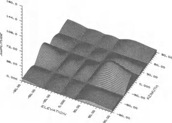
Figure 6.10 shows the steady-state adapted beam pattern for a 4 x 4 antenna array. The desired signal direction coincides with the antenna boresight, and a jammer with an interference-to-noise ratio (INR) of 40 dB is located at eo = 48°, and ea = _tOo. The quiescent pattern for an array with uniformly weighted elements is given in Fig. 6.11. The eigenbeam pattern corresponding to the interferer in Fig. 6.10 is given in Fig. 6.12. Figure 6. to was derived using the 2D Howells-Applebaum algorithm. The derivation of the 2D eigenbeam pattern is based on the procedure described in Sect. 6.3.2.4. In Fig. 6.12, it is observed that the main lobe of the eigenbeam pattern coincides with the AOA of the unwanted signal, and its amplitude is equal to the magnitude that the interfering signal would have if it were received by the quiescent pattern in Fig. 6.11. This results in a deep null in the direction of the interferer in Fig. 6.10. The interference null is further illustrated in Figs. 6.13a, b, which show cross sections through the interfering source along the elevation and azimuth planes. Note that a deep null is observed in both figures at the expected jammer location. These results support the contention made earlier that adaptive beamforming can be carried out by operating independently on the rows and columns of the 2D arrays.