

Diss / 10
.pdfSignal Processing by Digital Generalized Detector in Complex Radar Systems |
53 |
||||||||||||
|
|
ZDGDout (Nb) |
|
|
|
|
|
|
|
|
|
|
|
1.0 |
|
ZDGDout (∞) |
|
|
|
|
|
|
|
|
|
|
|
|
|
|
|
|
|
|
|
|
|
|
|||
|
|
|
|
|
|
|
|
|
|
|
|
|
|
0.9 |
|
|
|
|
|
|
|
|
|
|
|
|
|
0.8 |
|
|
|
|
|
|
|
|
|
|
|
|
|
0.7 |
|
|
|
|
|
|
|
|
1 |
|
|
|
|
0.6 |
|
|
|
|
|
|
|
Ts = |
|
|
|
|
|
|
|
|
|
|
|
|
2ΔF0 |
|
|
|
|||
0.5 |
|
|
|
|
|
|
|
|
|
|
|
||
|
|
|
|
|
|
|
|
|
|
|
|
|
|
0.4 |
|
|
|
|
|
|
|
|
|
|
|
|
|
0.3 |
|
|
|
|
|
|
|
|
|
|
|
|
|
0.2 |
|
|
|
|
|
|
|
|
|
|
|
|
|
0.1 |
|
|
|
|
|
|
|
|
|
|
|
|
|
0.0 |
|
|
|
|
|
|
|
|
|
|
|
Nb |
|
|
2 |
3 |
4 |
5 |
6 |
7 |
8 |
9 |
10 |
|
|||
|
|
|
|
||||||||||
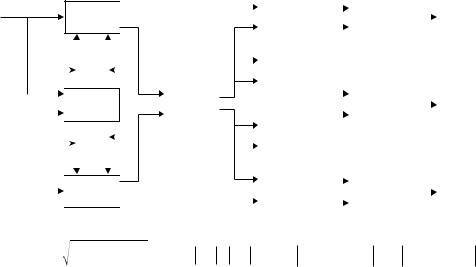
FIGURE 2.13 The DGD output signal amplitude ratio ZDGDout (Nb ) ZDGDout (∞) as a function of the digit capacity Nb of input signal.
least two times higher than the limiting sampling rate fsmax. There is a need to take into account the fact that an increase in the sampling rate fs causes a drastic increase in DGD design and realization complexity, that is, the technical specifications to required performance and memory size of digital signal processing equipment become rigid. For this reason, in the course of designing the DGD, it is recommended to choose the sampling rate fs within the limits 2 ÷ 3 F0.
The number of bits of the sampled target return signal or digit capacity sampling width plays a very important role in the definition of the DGD performance. Computer simulation results representing a DGD output signal amplitude ratio ZDGDout (Nb ) ZDGDout (∞) as a function of the digit capacity of the target return signal amplitude samples Nb are shown in Figure 2.13. Here ZDGDout (Nb ) denotes the DGD output signal at limited digit capacity Nb and ZDGDout (∞) denotes the GD output signal without sampling (Nb → ∞). As we can see from Figure 2.13, at Nb ≥ 10…12 a dependence of the DGD output signal amplitude peak on the digit capacity Nb is weak. Thus, this digit capacity Nb can be recommended under the DGD designing in digital signal processing subsystems of complex radar systems.
2.6 SUMMARY AND DISCUSSION
The discussion in this chapter allows us to draw the following conclusions.
Under the designing of analog-to-digital converters, the task of choosing a sampling interval value and the number of signal quantization levels of the sampled target return arises. Simultaneously, we should take into account the problems of designing and realization both for converters and for digital receivers processing the target return signals.
A sampling device can be considered as a make circuit with the time τ and sampling period Ts. The instantaneously sampled target return signal xδ(t) has a mathematical form similar to that of the Fourier transform of a periodic signal. Representation of the continuous function x(t) in the form of the sequence {x(nTs)} is possible only under well-known restrictions. One restriction in kind is a requirement of spectrum limitation of the sampled target return signal xδ(t). By Kotelnikov’s theorem concerning the signal space concept [4], the continuous target return signal x(t) possessing a limited spectrum is completely defined by a countable set of samples spaced Ts ≤ 1/(2fmax) seconds apart, where fmax is the cutoff frequency of target return signal spectrum.
The complex envelope of a narrowband radio signal can be presented either by the envelope and the phase, which are the functions of time, or by the in-phase and quadrature components.
54 |
Signal Processing in Radar Systems |
Accordingly, under the narrowband radio signal sampling there is a need to use two samples: either the envelope amplitude and the phase or the in-phase and quadrature components of complex amplitude of the narrowband radio signal. Thus, we deal with two-dimensional signal sampling.
Under digital signal processing of target return signals in CRSs there is a need to carry out a quantization of sampled values of complex envelope and phase or in-phase and quadrature components of radio signals in addition to sampling. Devices that carry out this function are called quantizers. We define the main parameters of the analog-to-digital conversion: sampling and quantization errors, reliability, that is, the ability to keep accuracy at given boundaries within the limits of definite time interval under a given environment, and other parameters producing a limitation in power consumption, weight and dimensions of analog-to-digital converters, cost under serial production, time that is required for design, and so on. We would like to pay attention to the following fact that there are two types of sampling and quantization errors: the dynamical errors and statical errors. The dynamical errors are the discrete transform errors. The statical errors are the unit sample errors. The dynamical errors depend on the target return signal nature and time performance of the analog-to-digital converter. The main constituent of this error is an inaccuracy caused by variations in the target return signal parameters at the analog-to-digital converter input.
The sampling and quantization techniques are used to digitize analog signals. For example, the sampling technique is used to discretize a signal within the limits of the time interval, and the quantization technique is used to discretize a signal by amplitude within the limits of the sampling interval. For this reason, there is a need to distinguish errors caused by these two digitizing techniques that allow us to obtain a high accuracy of receiver performance. Amplitude quantization and sampling can be considered as the additional noise ζ1(kTs) and ζ2(kTs) with zero mean and the finite variances σζ21 and σζ22, respectively. If the relationship between the chosen amplitude quantization step x and the mean square deviation σ′ of process at sampling, and quantization block output is determined by x < σ′, then the absolute value of mutual correlation function between the amplitude quantization error and the signal is approximately equal to 10−9 with respect to the values of the autocorrelation function of the signal. Therefore, it is reasonable to neglect this mutual correlation function. As a first approximation, it is reasonable to assume that the noise ζ1(kTs) and ζ2(kTs) are Gaussian.
In the case of the phase-code-manipulated target return signal, the DGD employed by a digital signal processing subsystem in a CRS uses only four convolving blocks. Moreover, a convolution within the limits of each cycle equal to the elementary signal duration τ0 is a summation of amplitude samples of the in-phase and quadrature constituents of the target return signal at instants with signs defined by values S*[i] = ±1 in accordance with the given code of the phase-manipulated operation. Practical realization of this principle is not difficult. In the considered case, a direct realization of convolution operations by serial digital signal processing techniques is not possible. There is a need to apply specific procedures of calculations under digital signal processing. First of all, we may use a principle of parallelism that is characteristic of convolution problems. This principle allows us to calculate n0 of pairwise multiplications S*[i] × x[k − (n0 − i)], where i = 1,…, n0, simultaneously using n0 parallel multipliers with subsequent summation of partial multiplications (see Figure 2.8). In this case, each multiplier must possess the processing speed Vreq = 5 × 10⁶ multiplications per second, that is, one multiplication operation per 40 ns. This processing speed can be easily provided by employing VLSI circuits. Another example of accelerated convolution operation is the implementation of specifically designed processor that uses the ROM blocks to store calculations of bitwise multiplications made before. Factor codes are used as result addresses of these bitwise multiplications.
Convolution of sequences in the frequency domain is reduced to a product of DFT results. For this purpose, there is a need to realize two DFTs, namely, to convolve a sequence of readings of the function {X[i]}, i = = 0, 1, 2,…, n − 1 and a sequence of readings of the impulse response of filters used by DGD. If after convolution it is necessary to make transformations into the time domain, there is a need to carry out IDFT for a sequence of spectral components {FX[k]}, k = 0, 1, 2,…, n − 1.
Signal Processing by Digital Generalized Detector in Complex Radar Systems |
55 |
The principal peculiarity of the considered algorithm of the operation DFT-Convolution-IDFT is a group technology type flow procedure if a width of input data array is higher n, that is, l ≥ n. The resulting convolution width is l + n − 1. In detection problems solved by DGD, we assume that the impulse response of all filters used by DGD is not variable, at least for probing signals of the same kind. Therefore, the DFT of impulse response of all filters used by DGD is carried out in advance and stored in the memory device of a corresponding computer. In the course of convolution, there is a need to accomplish one DFT and one IDFT. It must be emphasized that under radar detection and signal processing problems, a convolved sequence width L corresponds to radar range sweep length that is greater in comparison with the width of a convolving sequence equal to a width of impulse response nim of filters used by DGD.
Evaluation of the required memory size to realize the DGD in a radar signal processing subsystem under the implementation of FFT is based on the following statements. Using the same memory storage cells for FFT and IFFT and the buffer to store the output signal (see Figure 2.11), the memory size required for functional DGD purposes is Q = M1 + M2 + M3 + l, where M1 is the number of storage cells required for input sequence cells; M2 is the number of storage cells required for FFT and IFFT; M3 is the number of storage cells required for the spectral components of impulse responses of all filters used by DGD; l is the number of storage cells required for the output sequence. Thus, the use of FFT requires higher memory size compared to the implementation of FT in the frequency domain. A frequency of convolution operations can be essentially increased using a continuous-flow FFT system. In this case, the specific processor for FFT consists of 0.5M log2M devices for arithmetic operations functioning in parallel. Each arithmetic device fulfills a transformation at a definite stage of FFT. In doing so, we can reduce the calculation time in log2 0.5M times. The continuousflow FFT system requires additional memory in the form of interstage delay registers.
REFERENCES
1.Haykin, S. and M. Mocher. 2007. Introduction to Analog and Digital Communications. 2nd edn. New York: John Wiley & Sons, Inc.
2.Lathi, B.P. 1998. Modern Digital and Analog Communication Systems. 3rd edn. Oxford, U.K.: Oxford University Press.
3.Ziemer, R. and B. Tranter. 2010. Principles of Communications: Systems, Modulation, and Noise. 6th edn. New York: John Wiley & Sons, Inc.
4.Kotel’nikov, V.A. 1959. The Theory of Optimum Noise Immunity. New York: McGraw-Hill, Inc.
5.Manolakis, D.G., Ingle, V.K., and S.M. Kogon. 2005. Statistical and Adaptive Signal Processing. Norwood, MA: Artech House, Inc.
6.Goldsmith, A. 2005. Wireless Communications. Cambridge, U.K.: Cambridge University Press.
7.Kamen, E.W. and B.S. Heck. 2007. Fundamentals of Signals and Systems. 3rd edn. Upper Saddle River, NJ: Prentice Hall, Inc.
8.Tse, D. and P. Viswanath. 2005. Fundamentals of Wireless Communications. Cambridge, U.K.: Cambridge University Press.
9.Simon, M.K., Hinedi, S.M., and W.C. Lindsey. 1995. Digital Communication Techniques: Signal Design and Detection. 2nd edn. Upper Saddle River, NJ: Prentice Hall, Inc.
10.Richards, M.A. 2005. Fundamentals of Radar Signal Processing. New York: McGraw-Hill, Inc.
11.Oppenheim, A.V. and R.W. Schafer. 1989. Discrete-Time Signal Processing. New York: Prentice Hall, Inc.
12.Kay, S. 1998. Fundamentals of Statistical Signal Processing: Detection Theory. Upper Saddle River, NJ: Prentice Hall, Inc.
13.Tuzlukov, V. 1998. Signal Processing in Noise: A New Methodology. Minsk, Belarus: IEC.
14.Tuzlukov, V. 2001. Signal Detection Theory. New York: Springer-Verlag, Inc.
15.Tuzlukov, V. 2002. Signal Processing Noise. Boca Raton, FL: CRC Press.
16.Tuzlukov, V. 2005. Signal and Image Processing in Navigational Systems. Boca Raton, FL: CRC Press.
17.Tuzlukov, V. 1998. A new approach to signal detection theory. Digital Signal Processing, 8(3): 166–184.
18.Tuzlukov, V. 2010. Multiuser generalized detector for uniformly quantized synchronous CDMA signals in AWGN noise. Telecommunications Review, 20(5): 836–848.
56 |
Signal Processing in Radar Systems |
19.Tuzlukov, V. 2011. Signal processing by generalized receiver in DS-CDMA wireless communication systems with optimal combining and partial cancellation. EURASIP Journal on Advances in Signal Processing, 2011, Article ID 913189: 15, DOI: 10.1155/2011/913189.
20.Tuzlukov, V. 2011. Signal processing by generalized receiver in DS-CDMA wireless communication systems with frequency-selective channels. Circuits, Systems, and Signal Processing, 30(6): 1197–1230.
21.Tuzlukov, V. 2011. DS-CDMA downlink systems with fading channel employing the generalized receiver. Digital Signal Processing, 21(6): 725–733.
22.Papoulis, A. and S.U. Pillai. 2001. Probability Random Variables and Stochastic Processes. 4th edn. New York: McGraw-Hill, Inc.
23.Hayes, M.H. 1996. Statistical Digital Signal Processing and Modeling. New York: John Wiley & Sons, Inc.
24.Proakis, J.G. and D.G. Manolakis. 1992. Digital Signal Processing. 2nd edn. New York: Macmillan, Inc.
25.Kammler, D.W. 2000. A First Course in Fourier Analysis. Upper Saddle River, NJ: Prentice Hall, Inc.

3 Digital Interperiod Signal
Processing Algorithms
3.1 DIGITAL MOVING-TARGET INDICATION ALGORITHMS
The main fundamental theoretical principles of moving-target indication radar are delivered well in Ref. [1]. The performance of the moving-target indication radar can be greatly improved due primarily to four advantages:
•Increased stability of radar subsystems such as transmitters, oscillators, and receivers
•Increased dynamic range of receivers and analog-to-digital converters
•Faster and more powerful digital signal processing
•Better awareness of the limitations, and therefore requisite solutions, of the adapting moving-target indication radar systems to the environment
These four advantages can make it practical to use sophisticated techniques that were considered, and sometimes tried, many years ago but were impractical to implement. Examples of early concepts that were well ahead of the adaptive technology were the velocity-indicating coherent integrator [2] and the coherent memory filter [3,4].
Although such technological developments are able to augment the moving-target indication radar capabilities substantially, there are still no perfect solutions to all problems encountered with using moving-target indication radars, and the design of moving-target indication radar systems is still as much an art as it is a science. Examples of current problems include the fact that when receivers are built with increased dynamic range, limitations arising out of systemic instability will cause increased clutter residue (relative to system noise), leading to false detections. Clutter maps, which are used to prevent false detections from clutter residues, work quite well on fixed radar systems but are difficult to implement on, for example, shipboard radars, because as the ship moves, the aspect angle and range to each clutter patch changes, creating increased residues after the clutter map. A decrease in the resolution of the clutter map to counter the rapidly changing clutter residue will preclude much of the interclutter visibility, which is one of the least appreciated secrets of successful moving-target indication radar operation. The moving-target indication radar must work in the environment that contains strong fixed clutter; birds, bats, and insects; weather; automobiles; and ducting. The ducting is also referred to as anomalous propagation; it causes radar return signals from clutter on the surface of the Earth to appear at greatly extended ranges, which in turn exacerbates the problems with birds and automobiles, and can also cause the detection of fixed clutter hundreds of kilometers away.
3.1.1 Principles of Construction and Efficiency Indices
When signal processing is carried out under conditions of correlated passive interferences, an initial optimal signal processing of pulse train from N coherent pulses is reduced to ν-fold (ν ≤ N) interperiod subtraction of complex amplitude envelopes of the pulse train with subsequent accumulation of uncompensated remainders. A procedure of the interperiod subtraction (equalization) of fixed-position correlated interferences (interferences generated by fixed-position correlated sources) allows us to indicate targets moving relative to radar system. As a rule, this procedure is called the moving-target indication.
57
58 |
Signal Processing in Radar Systems |
About 25–30 years ago, the moving-target indication was carried out by analog wireless devices such as delay circuit, analog filters, and so on. Currently, digital moving-target indicators are widely used for the equalization of passive interferences. The digital moving-target indicators consist of memory devices and digital filters [5–8].
The designing of digital moving-target indicators and the evaluation of their efficiency must take into consideration the following peculiarities:
•Using the digit capacity Nb ≥ 8 of the target return signal amplitude samples in the digital moving-target indicator, quantization errors can be considered as the white Gaussian noise that is added to the receiver noise; on account of this, a synthesis of the digital movingtarget indicator is carried out using an analog prototype, that is, by the digitization of wellknown analog algorithms.
•Quantization of the target return signal amplitude samples leads to additional losses under the equalization of passive interferences, compared to that observed with the use of analog moving-target indicators.
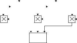
The digital moving-target indicators can be presented using both two-channel and single-channel forms. The block diagram of the two-channel digital moving-target indicator is shown in Figure 3.1. After processing by DGD, the in-phase and quadrature components of the DGD output signal come in at the inputs of two similar digital filters realizing the interperiod subtraction operation. Under single subtraction, the output signals of quadrature channels of the filter can be presented in the following form:
|
ZIout[i] = ZDGDout |
I [i] − ZDGDout |
I [i − 1] |
|
||
|
|
|
|
|
. |
(3.1) |
|
|
|
|
|
||
ZQout[i] = ZDGDout |
Q [i] − ZDGDout |
Q [i − 1] |
|
|||
|
|
|
|
|
|
|
In a similar manner, we can obtain the formulas for the filter output signals in the case of any ν-fold (ν ≤ N) interperiod subtraction when ν = 2, 3,…. There is a need to take into consideration that the operations are realized on the signals obtained within the limits of the same sampling interval under sampling in time and the index i denotes the current value of the sweep. Thus, the signals ZIout [i] and ZQout[i] are either accumulated at first and united after accumulation or are united at
Z outDGDI [i]
ISF-ν
|
Z DGDout |
I [i – 1] |
. . . . . |
|
||||
|
|
|
||||||
|
|
|
|
|
|
|
|
|
|
|
|
|
|
|
Memory |
||
|
|
|
|
|
|
|
device |
|
|
Z DGDout |
|
|
|
|
|||
|
|
|
|
|
|
|
||
|
Q[i – 1] |
|
|
|||||
|
|
|
|
|
|
|
. . . . . |
|
|
|
|
|
|
|
|
ISF-ν |
|
|
|
|
|
|
|
|
||
out |
[i] |
|
|
|
|
|||
|
|
|
|
|
|
|||
ZDGDQ |
|
|
|
|
|
|
||
|
|
|
Z Iout [i] = ZIouti |
|
|
|
|
|
|
|
|
|
|
|
|
|
|
|
|
||||||
|
(ZIouti )2 |
|
|
|
|
|
ZMTIout i |
|
|||||||||||||||||
|
|
|
|
|
|
|
|
|
|
|
|
|
|
|
|
||||||||||
|
|
|
|
|
|
|
|
|
|
|
|
|
|
|
|
||||||||||
|
|
|
|
|
|
|
|
|
|
|
|
|
|
|
|
|
|
|
|
|
|
|
|
|
|
|
|
|
|
|
|
|
|
|
|
|
|
|
|
|
|
|
|
|
|
|
|
|
|
|
|
|
|
|
|
|
|
|
|
|
Z out |
|
|
|
|
|
|
|
|
|
|
||||||
|
|
|
Z |
out [i – n + 1] |
|
|
|
|
|
|
|
|
|
|
|
|
|||||||||
|
|
|
|
|
|
|
|
|
|
|
|
|
|||||||||||||
|
|
|
|
|
|
|
|
|
|
|
I |
|
|
|
|
|
|
|
|
|
|
|
|
|
|
|
|
|
DGD1 |
|
|
|
i |
|
|
|
|
|
|
|
|
|
|
|
|
||||||
|
|
|
|
|
Coherent |
|
|
|
|
|
|
|
|
|
|
|
|
|
|
|
|
|
ZMTIout i |
|
|
|
|
|
|
|
|
|
|
|
|
|
|
|
|
|
|
|
|
|
|
|
|
|
|||
|
|
|
|
|
integrator |
|
|
|
|
|
|
|
|
|
|
|
|
|
|
|
|
|
|
||
|
|
|
Z |
out [i – n + 1] |
|
|
Z out |
|
|
|
|
|
|
|
|
|
|
||||||||
|
|
|
|
|
|
|
|
|
|
|
|
|
|||||||||||||
|
|
|
|
|
|
|
|
|
|
|
|
|
|
|
|||||||||||
|
|
|
|
|
|
|
|
|
|
|
|
|
|
|
|||||||||||
|
|
|
|
|
|
|
|
|
|
|
Q |
|
|
|
|
|
|
|
|
|
|
|
|
||
|
|
|
|
DGDQ |
|
|
|
|
|
|
i |
|
|
|
|
|
|
|
|
|
|
||||
|
|
|
|
|
|
|
|
|
|
|
|
|
|
|
|
|
|
|
|
|
|
||||
|
|
ZQout [i] =ZQout |
|
|
|
|
|
|
|
|
|
|
|
|
|
|
|
|
|
|
|
|
|||
|
|
|
|
|
|
(Z out)2 |
|
|
|
|
|
out |
|
||||||||||||
|
|
|
|
|
|
|
|
|
|
|
|||||||||||||||
|
|
|
|
|
|
|
|
|
|
|
|||||||||||||||
|
|
|
|
|
i |
|
|
|
|
|
Qi |
|
|
|
|
|
|
|
|
|
|
ZMTIi |
|
||
|
|
|
|
|
|
|
|
|
|
|
|
|
|
|
|
|
|
|
|
||||||
|
|
|
|
|
|
|
|
|
|
|
|
|
|
|
|
|
|
|
|
|
|
|
|
|
|
FIGURE 3.1 Flowchart of the two-channel digital moving-target indicator: ISF-ν–ν-fold interperiod sub-
traction filter; ZMTIout 1 = (ZIouti )2 + (ZQouti )2 ; ZMTIout 2 = ZIouti + ZQouti ; ZMTIout 3 = max(ZIouti , ZQouti ) + 0.5 min(ZIouti , ZQouti ).

Digital Interperiod Signal Processing Algorithms |
59 |
first and subjected to noncoherent accumulation before coming in at the input of decision circuit. Possible ways of packing of the in-phase and quadrature signal components are shown in Figure 3.1, the outputs 1, 2, and 3. The single-channel digital moving-target indicator can be obtained from a two-channel digital moving-target indicator version if only one of the channels of the two-channel digital moving-target indicator shown in Figure 3.1 is used. In this case, the block diagram of the digital moving-target indicator is significantly simplified, but additional losses in the SNR do occur.
In practice, the following indices are widely used for the evaluation of the efficacy of digital moving-target indicators:
•The coefficient of interference cancellation Gcan that is defined as a ratio of the passive interference power at the equalizer input to the passive interference power at the equalizer output
Gcan = |
Ppiin |
= |
σ2piin |
at σ2pi |
|
σ2n, |
(3.2) |
|
Ppiout |
σ2piout |
in |
||||||
|
|
|
|
|
where
Ppiin is the power of the passive interference at the equalizer input σ2piin is the variance of the passive interference at the equalizer input Ppiout is the power of the passive interference at the equalizer output
σ2piout is the variance of the passive interference at the equalizer output
σ2n is the receiver noise
•Figure of merit for the case of linear interperiod cancellation of the passive interferences can be defined in the following manner:
η = |
Psout /Ppiout |
= |
Psin |
× |
Psout |
= Gcan × Gs , |
(3.3) |
|
Psin /Ppiin |
Ppiout |
Psin |
||||||
|
|
|
|
|
where Gs is the coefficient characterizing a signal passing through the passive interferences equalizer. In general, when a nonlinear signal processing is used, the figure of merit η indicates to what extent the interference power at the equalizer input can be increased, without losses in detection performance.
•The coefficient of improvement is a characteristic of the response of the digital movingtarget indicator on passive interferences with respect to the averaged response on target return signals:
Pout /Pout
Gim = s pi , (3.4)
Psin /Ppiin Vtg
where [Psin /Ppiin]Vtg is the SNR at the equalizer input while deciding on the average values with respect to all target velocities.
The aforementioned Q-factors can be determined both for passive interferences equalizer systems using the interperiod subtraction and for equalizer systems with subsequent accumulation of residues after the passive interference cancellation.
60 |
Signal Processing in Radar Systems |
3.1.2 Digital Rejector Filters
The main element of the digital moving-target indicator is the digital rejector filter that can guarantee a cancellation of correlated passive interference. In the simplest case, the digital rejector filter is constructed in the form of the filter with the ν-fold (ν ≤ N) interperiod subtraction that corresponds to the structure of the nonrecursive filter. The recursive filters are also widely used for the cancellation of passive interferences. Consider briefly the problems associated with the analysis and synthesis of rejector filters.
The signal processing algorithm of the digital nonrecursive filter takes the following form:
ν |
|
ZIQoutnr (nT ) = ZIQoutnr [n] = ∑hiZIQin nr [n − i], |
(3.5) |
i= 0
where
hi is the weight coefficient of the filter
ZIQin nr [n − i] are in-phase and quadrature components of signal at the filter input (the DGD output)
At ν = 2, (3.5) defines a signal processing algorithm for the nonrecursive filter with the double interperiod subtraction. To define the coefficients of this filter we can set up the following equations:
ZIQoutnr [n] = ZIQin nr [n] − ZIQin nr [n − 1]; |
(3.6) |
ZIQoutnr [n − 1] = ZIQin nr [n − 1] − ZIQin nr [n − 2]; |
(3.7) |
ZIQoutnr [n] = ZIQoutnr [n] − ZIQoutnr [n − 1] = ZIQin nr [n] − 2ZIQin nr [n − 1] + ZIQin nr [n − 2]. |
(3.8) |
Consequently, the filter coefficients are equal to h0 = h2 = 1, h1 = −2, hi = 0 at i > 2. The flowchart of the digital filter with the interperiod subtraction at ν = 2, in the case of the single quadrature channel, is shown in Figure 3.2. Similarly, we can derive the filter coefficients at ν > 2. So, at ν = 3 we obtain h0 = 1, h1 = −3, h2 = 3, h3 = −1, hi = 0 at i > 3; and the signal processing algorithm takes the following form:
ZIQoutnr [n] = ZIQin nr [n] − 3ZIQin nr [n − 1] + 3ZIQin nr [n − 2] − ZIQin nr [n − 3]. |
(3.9) |
|||||||||||||||||||
|
|
|
|
|
|
Shift in frequency f = 1/Ts |
|
|
|
|
|
|||||||||
|
|
|
|
|
|
|
|
|
|
|
|
|
|
|
|
|
|
|
|
|
|
ZIinnr[n] |
|
|
|
|
|
|
|
|
|
|
|
|
|
|
|
|
|
||
|
|
|
|
|
|
|
|
|
|
|
|
|
|
|
|
|
|
|||
Memory |
|
|
|
|
|
|
Memory |
|
|
|
|
|
||||||||
|
|
|
|
|
device 1 |
|
|
|
|
|
|
device 2 |
|
|
|
|
|
|||
|
|
|
|
|
|
h0 = 1 |
|
|
|
|
|
|
h1 = –2 |
|
|
h2 = 1 |
|
|||
|
|
|
|
|
|
|
|
|
|
|
|
|
|
|
||||||
|
|
|
|
|
|
|
|
|
|
|
|
|
|
|
|
|
||||
|
|
|
|
|
|
|
|
|
|
|
|
|
|
|
|
|
|
|
|
|
|
|
|
|
|
|
|
|
|
|
|
|
|
|
|
|
|
|
|
|
|
Σ
 ZIoutnr [n]
FIGURE 3.2 Flowchart of the digital filter with the interperiod subtraction at ν = 2: the in-phase channel.
Digital Interperiod Signal Processing Algorithms |
61 |
The digital nonrecursive filters are very simple under realization, but they have very low-angle fronts of the amplitude–frequency performance, which severely affects the effectiveness of passive interference cancellation.
In addition to the nonrecursive filters, the recursive filter can be used as the rejector filter with the following signal processing algorithm:
ν |
ν |
|
|
ZIQoutnr [n] = ∑ai ZIQin nr [n − i] + ∑bj ZIQin nr [n − j], |
(3.10) |
||
i= 0 |
j = |
0 |
|
where ai and bj are the coefficients of the digital recursive filter.
Methods of recursive filter synthesis are considered and discussed in numerous literatures [9–21]. Without going into detail, we note that a synthesis procedure based on a squared amplitude– frequency filter response in accordance with a technique described in Ref. [22] can be considered the most effective for the digital moving-target indicators constructed based on the digital rejector filters. As a first step, and on the basis of the given parameters of environment conditions and initial premises, an order is chosen and the amplitude–frequency characteristic of analog filter prototype is defined. After that we define an approximation of squared amplitude–frequency characteristic of digital filter to the squared amplitude–frequency characteristic of analog filter-prototype, taking into consideration the restrictions arising from structural complexity. The elliptic filter, also known as Zolotaryov–Cauer filter [23], is best suited for these requirements.
Under realization of the digital rejector filter in accordance with (3.10), it is convenient that ai and bj are simple binary numbers. In this case, there is no need to use ROM to store these coefficients, and the multiplication operations are changed by simple shift and summation operations. For example, in the case of the recursive elliptic filter of the second order, synthesized using the squared amplitude– frequency characteristic, we obtain the following values of coefficients [22]: a0 = a2 = 1; a1 = −1.9682; b1 = −0.68; and b2 = −0.4928. To simplify the realization of the digital rejector filter, the coefficients a1, b1, and b2 can be rounded in the following order: a1 = −1.875 = −21 + 2−3, b1 = −0.75 = 20 + 2−3, b2 = −0.5 = −2−1. Investigations showed that rounding off of the coefficients a1, b1, and b2 can give a very small effect on the cancellation of passive interferences; however, this effect is negligible.
The digital rejector filter ensures the best cancellation of passive interferences due to an improvement in the amplitude–frequency characteristic shape, compared with the nonrecursive rejector filter of the same order. However, the degree of correlation of the passive interference remainders at the digital recursive filter output is higher compared to the correlation degree of the passive interference remainders at the digital nonrecursive filter. Moreover, the presence of positive feedback leads to an increase in the duration of transient process and corresponding losses in efficacy if the number of target return pulses in the train is less 20, that is, N < 20.
Now, consider some results of the comparison between the efficiency levels of the digital filter and the analog filter. At first, transform (3.10) to nonrecursive form, that is, present the signal processing algorithm of the digital recursive filter in the following form:
N −1 |
|
ZIQoutnr [n] = ∑hirf ZIQin nr [n − i], |
(3.11) |
i= 0 |
|
where |
|
N is the number of pulses in train (sequence) |
|
hirf are the coefficients of digital recursive filter impulse response defined by [23,24] |
|
k |
|
h0rf = 1, hirf = ai + ∑bjhi − jrf . |
(3.12) |
j =1
62 Signal Processing in Radar Systems
For example, in the case of the digital recursive second-order filter (ν = k = 2) we obtain h0rf = 1,
h1rf = a1 + h2rf = a2 + b1h1rf + b2, at i > 2 we have hirf = b1hi −1rf + b2hi − 2rf. As follows from (3.12), the impulse response of recursive filter tends to approach infinity and the number of used coefficients is
defined by the sample length of the input signal.
Efficiency of interperiod subtraction at different multiplicities of ν can be compared using the
coefficient of passive interference cancellation [25]: |
|
|
||
Gcan = |
|
1 |
, |
(3.13) |
|
|
|||
∑ν |
∑ν bihjρpi [(i − j)T ] |
|||
|
i= 0 |
j= 0 |
|
|
where |
|
|
|
|
ρpi[·] is the normalized coefficient of interperiod correlation of the passive interferences T is the radar bang period
At determination of Gcan for nonrecursive filters using (3.13) we think that ν is the multiplicity of the interperiod subtraction and for the recursive filters ν = Npi − 1, where Npi is the sample size of passive interferences.
To make calculations using (3.13) there is a need to define a model of interferences. The energy spectrum of passive interferences, that is, the signals reflected from, for example, extended territorial objects, clouds, or other types of reflectors, can be approximated by the Gaussian distribution law given by
|
|
|
Spi |
|
2 |
|
fpi (Spi ) ≈ exp |
−2.8 |
|
|
|
|
, |
|
||||||
|
|
|
fpi |
|
|
|
|
|
|
|
|
|
|
where
Spi is the energy spectrum of passive interferences
fpi is the bandwidth of passive interference spectrum at the level 0.5
The normalized coefficient of correlation corresponding to this spectrum is given as
|
|
π2 ( fpiiT )2 |
||
ρpi (iT ) = exp |
− |
|
. |
|
2.8 |
||||
|
|
|
||
(3.14)
(3.15)
Figure 3.3 represents the coefficient of passive interference cancellation Gcan as a function of fpiiT(i = 1) for various values of multiplicity of interperiod subtractions. As we can see from Figure 3.3, the use of the twofold interperiod subtraction brings a win in cancellation for about 15 dB compared to a single interperiod subtraction. In the case of the threefold interperiod subtraction, a win in cancellation in comparison with the twofold interperiod subtraction is less than 15 dB. In the case of the fourfold interperiod subtraction, a win in cancellation in comparison with the threefold interperiod subtraction is still less. The coefficient of cancellation of passive interferences for recursive filters depends on the sample size Npi of the passive interference. Thus, it is of no use to compare the recursive and nonrecursive filters by the coefficient of passive interference cancellation Gcan. Comparative efficacy of the interperiod subtraction and recursive filters can be evaluated by the figure of merit η given by (3.3), which corresponds to a win in SNR in
the case of digital linear filters.