

Diss / 10
.pdfDigital Interperiod Signal Processing Algorithms |
73 |
Further mathematical transformations of (3.50) are associated with an approximation of the function ln I0(x). In the case of weak signals, that is, qi 1, we use the following approximation
ln I0 |
2xiqi − xi2 |
+ xi2 |
≈ 1 xiqi2 |
− xi2 + xi2. |
(3.51) |
|
|
|
2 |
|
|
|
|
|
|
|
Consequently, taking into consideration that qi = q0gi and gi are the weight coefficients depending on the radar antenna directional diagram shape, the detection algorithm of weak target return pulse train will have the following form:
N |
|
|
|
|
|
|
|
|
|
ln Kg |
|
|
N |
|
|
2 2 |
4 |
4 |
|
|
|
|
|
2 |
|
2 |
|
||||
∑ |
2gi |
xi |
− xi |
i |
|
′ |
, where |
′ |
= |
|
+ 0.5q |
0 |
∑ |
gi . |
(3.52) |
2 |
|||||||||||||||
|
+ x |
|
≥ Kg |
Kg |
q0 |
|
|
||||||||
i=1 |
|
|
|
|
|
|
|
|
|
|
|
i=1 |
|
|
|
|
|
|
|
|
|
|
|
|
|
|
|
|
|
||
Now, consider the case of powerful signals, that is, qi 1. In this case, we use the following approximation:
ln I0 |
2xiqi − xi2 |
+ xi2 |
≈ 2xiqi − xi2 + xi2. |
(3.53) |
|
|
|
|
|
Consequently, taking into consideration that qi = q0gi and gi are the weight coefficients depending on the radar antenna directional diagram shape, the detection algorithm of powerful target return pulse train will have the following form:
N |
|
|
|
|
|
|
|
ln Kg |
|
N |
|
|
|
|
2 |
2 |
|
|
|
|
|
|
2 |
|
|
||
∑ |
2gi xi − xi |
i |
|
′ |
, where |
′ |
= |
|
0 |
∑ |
gi |
, |
(3.54) |
|
+ x |
|
≥ Kg |
Kg |
2q0 |
+ 0.5q |
|
||||||
i=1 |
|
|
|
|
|
|
|
|
i=1 |
|
|
|
|
|
|
|
|
|
|
|
|
|
|
|
|
Thus, in the case of the target return pulse train with completely known parameters and modulated by the radar antenna directional diagram, the generalized signal detection algorithm comes to weight summation of normalized samples of the target return pulse train and implementation of energy detector at the output of quadrature or linear detector within the limits of target return pulse
train bandwidth and comparison of accumulated statistic with the threshold K ′.
g
In practice, when the real radar system is employed, the target return pulse train contains the unknown parameters, such as SNR, that is, q0, at the maximum point of radar antenna directional diagram, the delay td of the target return pulse train relative to searching/scanning signal, and angular deflection of the target return pulse train center θ in the scanning plane with respect to the fixed direction θ0. Because of this, to process information completely inside the radar coverage a realization of generalized signal detection algorithm should be organized within the limits of each interval of time sampling or radar range discretization. Accumulation of processed signals must be carried out within the limits of “tracking/moving window.” The length of “tracking/moving window” must be equal to the number of target return pulses in train. In this case, at the low SNR (for rth sampling or discretization interval) the generalized detection algorithm of nonfluctuating target return pulse train (there are no fluctuations of the target reflecting surface) can be presented in the following form:
ln |
{ |
(r) |
} |
= |
N −1 |
2g2 |
|
x(r) |
2 − |
|
x(r) |
4 + |
|
x(r) |
4 ≥ K′ , r = 1, 2,…, M, |
M = |
T |
, µ ≥ N; (3.55) |
||
∑ |
( |
( |
( |
|
||||||||||||||||
|
g |
|
|
i |
µ −i ) |
|
µ −i ) |
|
µ −i ) |
|
g |
|
Ts |
|||||||
|
|
|
|
|
i= 0 |
|
|
|
|
|
|
|
|
|
|
|
|
|
||
74 |
Signal Processing in Radar Systems |
The generalized detection algorithm of fluctuating target return pulse train (there are fluctuations of the target reflecting surface) can be presented in the following form (at q0 1):
N −1 |
|
2g2k2 |
|
2 |
|
4 |
|
4 |
|
|
|
ln { (gr) } = ∑ |
i i |
|
(xµ(r−)i ) |
− (xµ(r−)i ) |
|
+ (xµ(r−)i ) |
|
|
≥ Kg′. |
(3.56) |
|
2 |
2 |
|
|
||||||||
i= 0 |
|
1 + gi ki |
|
|
|
|
|
|
|
|
|
In the case of powerful signal, the generalized signal detection algorithm within the limits of the “tracking/moving window” is obtained by analogous way. Thus, the DGD of target return pulse train with unknown parameters represents a composition of the “tracking/moving window” summator and energy detector with the threshold network and signal generator indicating a detection of the target return pulse train.
3.2.3 DGD for Binary Quantized Target Return Pulse Train
Now, consider the case when the input sequences are quantized on two levels by amplitude. The generalized detection algorithm of binary quantized target return pulse train is obtained from a synthesis of the likelihood ratio comparing it with the threshold. In doing so, we use the probability of signal detection PD and the probability of false alarm PF given by (3.43) and (3.44). The obtained generalized signal detection algorithm has the following form in its final version:
|
|
|
{ |
|
g |
} |
|
|
|
N −1 |
|
µ − |
|
′ |
|
|
||||
|
|
|
|
|
|
|
∑ |
|
|
|
|
|||||||||
|
|
ln |
|
|
(r) |
|
= |
|
|
|
χ jd(r)j |
≥ Kg |
, |
(3.57) |
||||||
|
|
|
|
|
|
|
|
|
|
|
j= 0 |
|
|
|
|
|
|
|
||
where the weight coefficients and the threshold are given by |
|
|
||||||||||||||||||
|
|
|
|
|
|
χ j = ln |
PSN bN |
; |
|
|
|
(3.58) |
||||||||
|
|
|
|
|
|
|
|
|
|
|
||||||||||
|
|
|
|
|
|
|
|
|
|
|
|
|
P b |
|
|
|
|
|||
|
|
|
|
|
|
|
|
|
|
|
|
|
|
N |
SN j |
|
|
|
|
|
|
|
|
|
|
|
|
|
|
|
|
|
|
|
|
N −1 b |
|
|
|
|
|
|
|
|
|
|
|
|
|
|
|
|
|
|
|
∑ bN |
|
|
||||
|
|
|
|
Kg = ln Kg − |
|
|
SN j |
; |
|
(3.59) |
||||||||||
|
|
|
|
|
′ |
|
|
|
|
|
|
|
|
|
|
|
|
|
|
|
|
|
|
|
|
|
|
|
|
|
|
|
|
|
|
j= 0 |
|
|
|
|
|
and |
|
|
|
|
|
|
|
|
|
|
|
|
|
|
|
|
|
|
|
|
|
∞ |
|
|
|
2 |
|
2 |
|
|
|
|
|
|
|
|
|
|
|||
|
|
|
|
|
|
|
|
|
|
|
|
|
|
|||||||
PSN j |
= ∫ xj exp − |
xj |
+ qj |
I0 (xj , qj )d(xj ); |
bSN j = 1 − PSN j |
(3.60) |
||||||||||||||
|
2 |
|
|
|||||||||||||||||
|
c0 |
|
|
|
|
|
|
|
|
|
|
|
|
|
|
|
|
|||
|
|
|
|
|
|
|
|
|
|
|
|
|
|
|
|
|
|
|
|
|
is the probability to get the unit on the jth position of the target return pulse train; |
|
|||||||||||||||||||
|
|
∞ |
|
|
|
|
|
|
|
2 |
|
|
|
|
|
|
|
|
||
|
|
|
|
|
|
|
|
|
|
|
|
|
|
|
|
|||||
|
|
PN = ∫ xj exp − |
xj |
d(xj ); |
bN = 1 − PN |
(3.61) |
||||||||||||||
|
|
|
||||||||||||||||||
|
|
c0 |
|
|
|
|
|
|
|
2 |
|
|
|
|
|
|
|
|
||
|
|
|
|
|
|
|
|
|
|
|
|
|
|
|
|
|
|
|
|
|
is the probability to get the unit in noise region (a “no” signal); |
|
|
||||||||||||||||||
|
|
|
|
|
|
|
1, |
|
if |
|
zin |
≥ c |
|
|
||||||
|
|
|
|
|
|
|
|
|
|
|
|
|
|
|
µ − j |
0 |
|
|
||
|
|
dµ − j |
= |
|
|
|
|
|
|
|
|
|
, |
|
(3.62) |
|||||
|
|
|
|
|
|
|
0, |
if |
|
zin |
< c |
|
|
|||||||
|
|
|
|
|
|
|
|
|
|
|
|
|
|
|
µ − j |
0 |
|
|
||
where c0 is the normalized threshold for binary signal quantization by amplitude.
Digital Interperiod Signal Processing Algorithms |
75 |
Thus, the generalized signal detection algorithm for the binary quantized target return pulse signals comes to summation of the weight coefficients χj corresponding to positions of the target return pulse train where dµ(r−) j = 1. The generalized signal detection algorithm of nonmodulated target return pulse train (in the case of scanning with the fixed antenna) takes the following form:
|
{ |
gµ } |
|
N −1 |
|
µ − j |
′′ |
|
|
|
∑ |
|
|
||||
ln |
|
|
= |
|
d |
|
≥ Kg. |
(3.63) |
j= 0
In other words, the generalized signal detection algorithm is reduced to accumulation of units within the limits of the target return pulse train length (within the limits of length of the “moving/ tracking window” with the predetermined sampling increment) and comparison of the obtained end sum with the threshold.
3.2.4 DGD Based on Methods of Sequential Analysis
The use of methods of the sequential analysis takes a very important place in signal detection theory. Detectors constructed based on methods of the sequential analysis allow us to determine the logarithm of likelihood ratio by the following recurrence formula [70–75]
ln { gµ } = ln { gµ−1 }+ ln { gµ }, |
(3.64) |
where
gµ−1 is the accumulated likelihood ratio over μ − 1 steps
g is the likelihood ratio increment at the μ-th step of sequential analysis
The accumulated step-to-step statistic ln{ g } is compared with the upper ln A and lower ln B thresholds
ln A = ln |
PD |
and ln B = ln |
1 − PD , |
(3.65) |
|
PF |
|||||
|
|
1 − PF |
|
where
PD is the predetermined probability of detection
PF is the predetermined probability of false alarm, correspondingly
If following a comparison we have
ln { g }≥ ln A, |
(3.66) |
the decision about signal detection is accepted and we stop analysis. If following a comparison we obtain
ln { g }≤ ln B. |
(3.67) |
Then the decision about a “no” signal is accepted and we also stop analysis. If the following condition is satisfied
ln B < ln { g }< ln A, |
(3.68) |

76 |
Signal Processing in Radar Systems |
In{ |
g } |
Decision a “yes” signal |
|
In A |
|
|
|
|
|
In{Δ |
g} |
0 |
|
|
|
–1 |
|
|
|
|
|
|
|
In B |
|
|
|
|
|
Decision a “no” signal |
|
FIGURE 3.7 Accumulation of statistic and decision-making procedure under the sequential analysis.
we continue an analysis, that is, we observe a new sample and determine the likelihood increment. The process of accumulation of ln{ g } and making a decision is presented in Figure 3.7.
Logarithm of likelihood increment is determined by the following formula:
ln { |
g } = ln |
pSN (x ) |
. |
(3.69) |
|
||||
|
|
pN (x ) |
|
|
In doing so, in the case of nonfluctuating target return pulse train model (there are no fluctuations of the target reflecting surface), we use the following logarithm of likelihood increment:
ln { |
g } = ln I0 |
(x , q ) − |
q2 |
. |
(3.70) |
|
|||||
|
|
2 |
|
|
|
In the case of rapidly fluctuating target return pulse train model (there are fluctuations of the target reflecting surface), we use the following logarithm of the likelihood increment:
ln { |
g |
|
} = |
|
k2 x2 |
− ln (1 + k2 ), |
(3.71) |
|
|
1 − k2 |
|||||||
|
|
|
|
|
||||
where the parameter k is given by (3.42).
Thus, to realize a procedure of sequential signal detection there is a need to first define the expected SNR by voltage, for example, in the case of nonfluctuating target return pulse train model (there are no fluctuations of the target reflecting surface), and by power in the case of rapidly fluctuating target return pulse train model (there are fluctuations of the target reflecting surface). The
main characteristic of sequential analysis procedure is the average number of steps – to make a final n
decision a “yes” or a “no” signal in the input process. Consider how the average number of steps depends on a “yes” signal and threshold under decision making.
In the case of a “no” signal in the input process, the procedure of sequential analysis is finished by the likelihood ratio logarithm ln{ g } overrunning the lower threshold ln B. Value of the lower threshold ln B does not depend on the predetermined probability of false alarm PF since the probability of false alarm PF varies within the limits of 10−3 ÷ 10−11 and is only defined by an acceptable
Digital Interperiod Signal Processing Algorithms |
77 |
value of the probability of miss, that is, PM = 1 − PD, where PD is the probability of signal detection. By this reason, the average cycle of sequential analysis procedure, in the case of a “no” signal in the input process, depends only on the predetermined probability of signal detection PD and increases with increasing in PD.
In the case of a “yes” signal at the DGD input, the procedure of sequential analysis is finished, as a rule, by overrunning the upper threshold ln A. A value of the upper threshold ln A is defined by the predetermined probability false alarm PF. Consequently, the average cycle of analysis in the case of a “yes” signal at the DGD input depends on the predetermined probability of false alarm PF and SNR.
An advantage of the DGD based on the sequential analysis in comparison with the well-known
Neyman–Pearson detector consists of the average number of target return signal samples –, which n
is necessary to make a decision based on the predetermined probability of false alarm PF and probability of signal detection PD is less under sequential analysis procedure than the fixed number of samples N required for the Neyman–Pearson detector. Consequently, it is possible to reduce the computer cost and power energy of a CRS under the detection of target. This possibility can be realized by a radar system with programmable radar antenna scanning when the radar antenna beam can be delayed in scanning direction until the end decision making. However, this advantage has been proved rigorously only in the case of a single channel, that is, under signal detection within the limits of a single radar range resolution interval. In the time of radar signal processing, there is a need to make a decision taking into consideration all elements of radar range resolution simultaneously (multichannel case). In this case, the effectiveness of sequential analysis is defined by the average number of searching radar signals required to make the end decision in all elements of radar range resolution with the predetermined probability of false alarm PF and probability of signal detection PD. This number is determined by the following formula:
n = max nk , |
(3.72) |
k=1,m |
|
where
m is the number of analyzed resolution elements in radar range
– is the average cycle of sequential analysis at the th radar range resolution element nk k
Optimality of sequential procedure in the multichannel radar systems is not proved so far. There are no analytical and theoretical methods and procedures to determine the efficacy of detectors constructed based on the sequential analysis and employed by multichannel radar systems. This is also particularly true for the DGD. For this reason, an analysis of the multichannel radar systems implementing the sequential analysis procedures is carried out using simulation techniques in each particular case. In what follows, we present some results of this analysis.
In the time of sequential analysis in the multichannel radar system there are two possible types of procedures:
•Decision making is an independent procedure: In this case, a test for the given channel is finished after reaching one of the thresholds—the upper threshold or the lower threshold.
•Simultaneous decision making: This decision making is made if all values of partial likelihood ratios overrun one of the thresholds—the upper threshold or the lower threshold. In this case, multiple crossings of the thresholds are possible.
The average number of tests both for the first case and for the second cases is defined by (3.72). However, the procedure of the second kind is more cost-effective in terms of the required average number of tests since this procedure allows us to level out the lower threshold and, consequently, decrease an uncertainty zone between the upper and lower thresholds. This statement is illustrated in Figure 3.8, where the lower threshold values are demonstrated to make a decision at the

78 |
|
|
|
|
|
|
|
|
|
Signal Processing in Radar Systems |
|||
In B |
|
|
|
|
|
|
|
|
|
|
|||
|
|
|
PD = 0.7 |
|
|
|
|
|
|
||||
|
|
|
|
|
|
|
|||||||
|
|
|
PF = 0.001 |
|
|
|
|
4 |
|
||||
|
|
|
|
|
|
|
|
|
|
|
|
|
|
|
|
|
|
|
|
|
|
|
|
|
|||
|
|
|
1 |
SNR = 0.5 |
|
|
|
|
3 |
|
|||
|
|
|
2 |
SNR = 1.5 |
|
|
|
|
|
||||
|
|
|
|
|
|
|
|
||||||
|
|
3 |
SNR = 3.0 |
|
|
|
|
|
|
||||
|
|
4 |
SNR = 4.0 |
|
|
|
|
2 |
|
||||
|
|
|
|
|
|
|
|
|
|
|
|
|
|
|
|
|
|
|
|
|
|
|
|
|
|
1 |
|
0 |
|
|
|
|
|
|
|
|
|
|
|
|
Ig m |
|
|
|
|
|
|
|
|
|
|
|
|
||
|
|
|
|
|
|
|
2 |
3 |
|
||||
|
|
|
|
|
1 |
|
|
|
|||||
In B1 |
|
|
|
|
|
|
|
|
|
|
|
|
|
|
|
|
|
|
|
|
|
|
|
|
|
|
|
FIGURE 3.8 Simultaneous decision making for multiplicity channel radar systems.
predetermined probability of false alarm PF = 10−3 and the probability of signal detection PD = 0.7 for various values of SNR under various ratios of the rapidly fluctuating target return pulse train model (there are fluctuations of the target reflecting surface) to the noise by power as a function of the number m (the number of analyzed resolution elements in radar range). As we can see from Figure 3.8, the value of the lower threshold increases with a corresponding increase in the SNR and m. In this case, at fixed values of the lower threshold, the probability of missing PM of the target return signal decreases inversely to the number m of analyzed resolution elements in radar range; however, in the case of sequential analysis procedure of the first kind, the probability of missing PM of the target return signal is independent of the number m of analyzed resolution elements in radar range.
In the case of a “no” signal at the DGD input, the average number of tests at sequential analysis procedure in a single receiver antenna radar system depends only on the predetermined probability of signal detection PD. In the multichannel radar system, there is a dependence of the average number of tests at sequential analysis procedure both on the predetermined probability of signal detection PD and on the number m of analyzed resolution elements in the radar range. Dependences between the average number of tests at sequential analysis procedure and the predetermined probability of signal detection PD, the probability of false alarm PF, and (SNR)2 = 1.5 obtained by simulation are presented in Figure 3.9. The average number of tests for a Neyman–Pearson detector are denoted by horizontal lines for each pair of the predetermined probability of signal detection PD and the probability of false
– |
0 |
|
|
|
|
|
|
|
|
|
|
ng |
|
|
|
|
|
|
|
|
|
||
80 |
|
|
|
|
|
|
|
|
|
3 |
|
|
|
|
|
|
|
|
|
|
|
||
|
|
1 |
PD = 0.5 |
|
|
|
|
|
|||
70 |
|
|
|
|
|
|
|
||||
|
|
|
|
|
|
|
|
||||
|
|
2 |
PD = 0.7 |
|
|
|
|
|
|
||
|
|
|
|
|
|
|
|||||
60 |
|
|
3 |
PD = 0.9 |
|
|
|
|
2 |
|
|
|
|
|
|
|
|
||||||
|
|
|
|
|
|
|
|
|
|||
50 |
|
|
|
|
|
|
|
|
|
3 |
|
40 |
|
|
|
|
|
|
|
|
|
1 PF = 10–9 |
|
|
|
|
|
|
|
|
|
|
|||
30 |
|
|
|
|
|
|
|
|
|
2 |
|
|
|
|
|
|
|
|
|
|
1 |
|
|
|
|
|
|
|
|
|
|
|
|
||
20 |
|
|
|
|
|
|
|
|
|
3 |
|
10 |
|
|
|
|
|
|
|
|
|
2 PF = 10–3 |
|
|
|
|
|
|
|
|
|
|
1 |
|
|
|
|
|
|
|
|
|
|
|
|
||
0 |
|
|
|
|
|
|
|
|
|
|
Ig m |
|
|
|
|
|
|
|
|
|
|
||
|
|
|
1 |
2 |
3 |
|
|||||
|
|
|
|
|
|
||||||
FIGURE 3.9 Average numbers of tests at the sequential analysis versus the number of resolution elements.
Digital Interperiod Signal Processing Algorithms |
79 |
alarm PF. The points of intersections of corresponding curves allow us to define the number of analyzed resolution elements in radar range at which the average number of tests for a Neyman–Pearson detector and the average number of tests for the DGD based on sequential analysis procedure is the same. Evidently, the DGD based on sequential analysis procedure is more effective in comparison with the Neyman–Pearson detector if the following condition in the case of a “no” signal
ng 0 |
< n 0 |
(3.73) |
seq |
N− P |
|
is satisfied. As follows from Figure 3.9, in the case of a “no” signal at the DGD input the efficacy of the DGD based on sequential analysis procedure is higher, and the predetermined probability of false alarm PF is lower. For a fixed value of the probability of false alarm PF the efficacy of the DGD based on sequential analysis procedure for m receiver antennas increases concomitant to decrease in the probability of signal detection PD.
In the multichannel radar systems, the average number of tests at sequential analysis procedure in the direction of target presence becomes commensurable with the average number of tests at sequential analysis procedure in the direction of target absence even at small numbers of resolution elements. Consequently, the average number of tests at sequential analysis procedure before a decision making is mainly defined by the average number of tests at sequential analysis procedure in the direction of target absence. In the multichannel radar systems, the average number of tests at sequential analysis procedure can be prolonged to such limits that are not acceptable by energy or other tactical considerations. The only way to avoid this prolonged delay of antenna beam in scanning direction is to introduce a truncation procedure of sequential analysis at the ntr-th step and to make a decision about exceeding some fixed threshold C. In this case, the probability of error at the truncation procedure can be presented in the following form:
Pertr = Per (n < ntr ) + Per (C)[1 − Per (n < ntr )], |
(3.74) |
where
(– ) is the probability of wrong decision at sequential analysis procedure before truncation
Per n < ntr
Per(C) is the probability of wrong decision at sequential analysis procedure under comparison of decision statistic with the threshold C
Obviously, we can choose such values of ntr and C that additional errors caused by truncation will be satisfied to the following conditions:
PF (C) ≤ PFadd er − PF (n < ntr ), |
(3.75) |
PM (C) ≤ PMadd er − PM (n < ntr ). |
(3.76) |
Algorithm to choose ntr and C satisfying to the conditions (3.75) and (3.76) comes to the following procedure: At n = ntr1, we can choose C such that the first condition given by (3.75) is satisfied. If, at the same time, the second condition given by (3.76) is also satisfied, we stop the procedure of choice. If the (3.76) is not satisfied, we select ntr2 = ntr1 +1 and test conditions (3.75) and (3.76) again. As was proved by the theory of sequential analysis [25,71], there are the required ntr and C. Introduction of truncation does not effect essentially the average number of tests at sequential analysis procedure in the direction of target absence and slightly reduces the average number of tests at sequential analysis procedure in the direction of target presence.
At binary quantization of the target return pulse train samples, the generalized detection algorithm based on the sequential procedure becomes essentially simple, but the efficacy of detection
80 |
Signal Processing in Radar Systems |
procedure is decreased. In this case, additional losses in the average number of tests at the sequential analysis procedure can be 15% ÷ 30%. Losses caused by quantization can be reduced to 2%/5% even at 7–8 quantization levels. This fact gives us a reason to design and construct the DGDs based on the sequential analysis procedure with small digit capacity of the target return pulse train samples.
Comparative analysis of effectiveness of the DGD based on the sequential analysis procedure and a detector with the fixed sample volume, for example, the Neyman–Pearson detector, gives rise to a consideration of two-stage signal detection procedure. The two-stage signal detection procedure consists of the following. At first, the target return pulse train sample with the fixed volume n1 is subjected to the generalized signal processing algorithm with the predetermined probability of signal detection PD1 and the probability of false alarm PF1. If the decision a “no” signal is made, the procedure is stopped. Otherwise, an additional procedure is carried out with respect to “suspect data,” and we use for this purpose n2 samples of the target return pulse train and obtain the probability of signal detection PD2 and the probability of false alarm PF2. In doing so, using results of the two stages, we obtain
PD = PD1 PD2 and PF = PF1 PF2 . |
(3.77) |
To solve the problem of optimization for the two-stage procedure we can choose such values of n1 and n2 that the average number of tests at sequential analysis procedure would be minimal. In doing so,
|
1 |
1 |
; |
|
|
n |
|
= n1 + PDn2 |
(3.78) |
||
|
|
|
|
|
|
|
|
|
|
|
|
|
0 |
0 |
, |
|
|
n |
|
= n1 + Psc′ n2 |
|
|
|
where at PF1 1 the probability of duplicate scanning in the a “no” signal direction is defined in the following form:
′ |
( |
1 ) |
1 1 |
|
|
Psc = |
1 |
− PF |
m1 ≈ m PF |
; |
(3.79) |
where
PF1 is the probability of false alarm at the first stage
n 1 is the average number of tests at sequential analysis procedure in the direction of target presence
n 0 is the average number of tests at sequential analysis procedure in the direction of target absence
n2 1 is the average number of tests at sequential analysis procedure in the direction of target presence at the second stage
n2 0 is the average number of tests at sequential analysis procedure in the direction of target absence at the second stage
m1 is the number of analyzed resolution elements in radar range at the first stage.
Two-stage DGD based on the sequential analysis procedure allows us to obtain an advantage from 25% to 40% in the average number of tests at sequential analysis procedure in comparison with the DGD or Neyman–Pearson detector with the fixed number of tests subjected to the predetermined probability of signal detection PD and the probability of false alarm PF. Under target detection at high values of the probability of false alarm PF, for example, PF = 103, and at large number of resolution elements, the two-stage DGD can be more effective in comparison with the DGD based on the sequential analysis procedure.

Digital Interperiod Signal Processing Algorithms |
81 |
3.2.5 Software DGD for Binary Quantized Target Return Pulse Train
In practice, while designing the detectors for binary quantized target return pulse train, many heuristic methods are used that make a decision about signal detection based on the definition of a unit density within the limits of each sampling interval of the target return pulse train at the envelope detector output. The best-known digital signal processing algorithms from this class of detectors are software algorithms fixing an initial instant of target return pulse train appearance by the presence of l units on m adjacent positions, where l ≤ m, m ≤ 5…10. This is the so-called criterion “l from m” or “l/m.” Criterion of the initial instant fixation of target return pulse train appearance is, at the same time, a criterion of target return pulse train detection. To eliminate ambiguity, a criterion of target return pulse train end is defined under an angular coordinate reading. As a rule, the target return pulse train end is fixed by presence of series from k skipping (zeros) one by one (k = 2…3). To determine positions between the origin and the end of target return pulse train the binary scalers are employed.
Each of the considered operations can be realized by the digital finite-state automaton. Composition of these digital finite-state automata gives us an example of the software detector block diagram presented in Figure 3.10, where A1 is the digital finite-state machine realizing the detection criterion “l/m”; A2 is the digital finite-state automaton realizing the criterion of target return pulse train end definition based on series from k zeros; and A3 is the digital finite-state automaton (counter) to determine the number of positions from the instant of target return pulse train detection to the instant of erasing the stored information. Using the well-known methods of abstract digital automata composition [76,77], we are able to obtain the transition matrix and graph of associated automaton realizing a program “l/m − k” for each data pattern l, m, and k. This graph is a starting point to design tools to realize the required digital signal detection algorithm, and the transition matrix allows us to determine rigorously the quality characteristics of software detectors.
Digital storage devices of binary quantized target return pulse train are considered as other groups of detection algorithms for software detectors. The origin of target return pulse train is fixed by the digital storage device by the first unit obtained after counter storage erasing. The target return pulse train end is fixed when a series of k zeros appears, that is, the same principle as for the software detectors. The signal detection is fixed at the instant of counter erasing if the number of storage units is equal or greater than the threshold Nthr. Storage devices of other types are designed in such a way that the counter stores the number of positions (cycles) within the limits of the target return pulse train bandwidth, not the number of units between series from k and more skipping one by one. In doing so, skipping of units at intrinsic positions of target return pulse train is restored. These storage devices are very convenient to realize a digital signal processing algorithm to define the angle coordinate reading of target return pulse train.
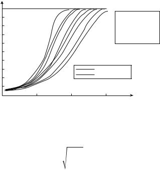
Analysis of quality characteristics of the digital software detectors and storage devices can be carried out both by analytic–theoretical method and by simulation. As an example, Figure 3.11 represents the detection performance of software detectors “3/3 − 2,” “3/4 − 2,” and “4/5 − 2” and digital storage device of units at the predetermined probability of false alarm PF = 10−4 for the target return pulse train consisting of 15 pulses modulated by the radar antenna directional diagram envelope of the following form:
|
|
|
|
g(x) = |
sin x |
. |
(3.80) |
|||||
|
|
|
|
|
|
|
x |
|
|
|
|
|
|
|
|
|
|
|
|
|
|
|
|
Nthr |
|
di |
|
|
|
A1 |
|
|
|
|
|
A3 |
||
|
|
|
|
|
|
|
|
|
|
|||
|
|
|
|
|
|
|
|
|
|
|
|
|
|
|
|
|
|
|
|
|
|
|
|
|
|
|
|
|
|
|
|
|
|
|
|
|
|
|
|
|
|
|
A2 |
|
|
|
|
|
|
|
|
|
|
|
|
|
|
|
|
|
|
|
|
|
|
|
|
|
|
|
|
|
|
|
|
|
|
FIGURE 3.10 Software detector block diagram.
82 |
Signal Processing in Radar Systems |
PD |
|
|
|
|
|
|
|
1.0 |
|
1 |
2 3 4 |
3 2 |
1 |
4 |
|
0.9 |
|
|
|
|
|
1 |
Digital storage |
0.8 |
|
|
|
|
|
2 |
device of units |
|
|
|
|
|
“4/5 – 2” |
||
0.7 |
|
|
|
|
|
3 |
“3/4 – 2” |
0.6 |
|
|
|
|
|
4 |
“3/3 – 2” |
|
|
|
|
|
|
|
|
0.5 |
|
|
|
|
|
|
|
0.4 |
|
|
|
|
|
|
|
0.3 |
|
|
|
Nonfluctuated |
|||
0.2 |
|
|
|
Fluctuated |
|
||
0.1 |
|
|
|
|
|
|
|
0.0 |
2 |
3 |
|
|
4 |
|
SNR (dB) |
1 |
|
|
|
|
|||
FIGURE 3.11 Detection performance of software detector.
Thresholds of binary quantization are determined by procedures discussed in Ref. [77,78]. The storage device detection threshold (the counter threshold) Nthr is determined in the following form:
|
N |
|
|
|
|
|
|
, i = {1, 2,…,15}. |
(3.81) |
Nthr = entier 1.5 |
∑gi |
|||
|
i=1 |
|
|
|
|
|
|
|
|
Simulation brings the following results:
•In the case of absence of target reflecting surface fluctuations under detection of the target return pulse train, the storage devices are more effective in comparison with the software detectors and vice versa; in the case of presence of target reflecting surface fluctuations under detection of the target return pulse train, the software detectors with the detection criterion “l/m” or “l < m” are more effective in comparison with the storage devices.
•Threshold losses are low when the target return pulse train is detected by “tracking/moving window” using both the software detectors and the storage devices. Digital realization of these detectors is sufficiently simple, which makes it advantageous to use these detectors when requirements for simplicity of realization prevail over requirements in minimization of energy losses.
•It is appropriate to employ the software detectors on the first stage under the two-stage detection procedure.
3.3 DGD FOR COHERENT IMPULSE SIGNALS WITH UNKNOWN PARAMETERS
3.3.1 Problem Statements of Digital Detector Synthesis
The synthesis problems of optimal detectors are solved with an assumption that there is a priori all information about the noise and interference and their statistical parameters and features under a predetermined energy and statistical characteristics of the target return signal (the information signal). The optimal signal processing and detection algorithms obtained under these conditions possess the best performance for established initial conditions. Changes in noise environment or deviation from characteristics considered under synthesis of detectors leads, as a rule, to a drastic decrease in the efficacy of signal processing and detection algorithms and even to losses in capacity for work.
Detection of target return signals by CRSs in practice is characterized by ambiguity, to a greater or lesser extent, in energy and statistical parameters of signals and noise. In addition, these