

Diss / 10
.pdfDigital Interperiod Signal Processing Algorithms |
113 |
50.Tuzlukov, V.P., Yoon, W.-S., and Y.D. Kim. 2004. Wireless sensor networks based on the generalized approach to signal processing with fading channels and receive antenna array. WSEAS Transactions on Circuits and Systems, 10(3): 2149–2155.
51.Kim, J.H., Tuzlukov, V.P., Yoon, W.-S., and Y.D. Kim. 2005. Performance analysis under multiple antennas in wireless sensor networks based on the generalized approach to signal processing. WSEAS Transactions on Communications, 7(4): 391–395.
52.Kim, J.H., Tuzlukov, V.P., Yoon, W.-S., and Y.D. Kim. 2005. Macrodiversity in wireless sensor networks based on the generalized approach to signal processing. WSEAS Transactions on Communications, 8(4): 648–653.
53.Kim, J.H., Tuzlukov, V.P., Yoon, W.-S., and Y.D. Kim. 2005. Generalized detector under no orthogonal multipulse modulation in remote sensing systems. WSEAS Transactions on Signal Processing, 2(1): 203–208.
54.Tuzlukov, V.P. 2009. Optimal combining, partial cancellation, and channel estimation and correlation in DS-CDMA systems employing the generalized detector. WSEAS Transactions on Communications, 7(8): 718–733.
55.Tuzlukov, V.P., Yoon, W.-S., and Y.D. Kim. 2004. Adaptive beam-former generalized detector in wireless sensor networks, in Proceedings of IASTED International Conference on Parallel and Distributed Computing and Networks (PDCN 2004), February 17–19, Innsbruck, Austria, pp. 195–200.
56.Tuzlukov, V.P., Yoon, W.-S., and Y.D. Kim. 2004. Network assisted diversity for random access wireless sensor networks under the use of the generalized approach to signal processing, in Proceedings of the 2nd SPIE International Symposium on Fluctuations in Noise, May 25–28, Maspalomas, Gran Canaria, Spain, Vol. 5473, pp. 110–121.
57.Tuzlukov, V.P., Yoon, W.-S., and Y.D. Kim. 2005. MMSE multiuser generalized detector for no orthogonal multipulse modulation in wireless sensor networks, in Proceedings of the 9th World Multiconference on Systemics, Cybernetics, and Informatics (WMSCI 2005), July 10–13, Orlando, FL. (CD Proceedings)
58.Kim, J.H., Tuzlukov, V.P., Yoon, W.-S., and Y.D. Kim. 2005. Collaborative wireless sensor networks for target detection based on the generalized approach to signal processing, in Proceedings of International Conference on Control, Automation, and Systems (ICCAS 2005), June 2–5, Seoul, Korea. (CD Proceedings)
59.Tuzlukov, V.P., Chung, K.H., and Y.D. Kim. 2007. Signal detection by generalized detector in com- pound-Gaussian noise, in Proceedings of the 3rd WSEAS International Conference on Remote Sensing (REMOTE’07), November 21–23, Venice (Venezia), Italy, pp. 1–7.
60.Tuzlukov, V.P. 2008. Selection of partial cancellation factors in DS-CDMA systems employing the generalized detector, in Proceedings of the 12th WSEAS International Conference on Communications, July 23–25, Heraklion, Creete, Greece. (CD Proceedings)
61.Tuzlukov, V.P. 2008. Multiuser generalized detector for uniformly quantized synchronous CDMA signals in wireless sensor networks with additive white Gaussian noise channels, in Proceedings of the International Conference on Control, Automation, and Systems (ICCAS 2008), October 14–17, Seoul, Korea. pp. 1526–1531.
62.Tuzlukov,V.P. 2009. Symbol error rate of quadrature subbranch hybrid selection/maximal-ratio combining in Rayleigh fading under employment of generalized detector, in Recent Advances in Communications: Proceedings of the 13th WSEAS International Conference on Communications, July 23–25, Rodos (Rhodes) Island, Greece, pp. 60–65.
63.Tuzlukov, V.P. 2009. Generalized detector with linear equalization for frequency-selective channels employing finite impulse response beamforming, in Proceedings of the 2nd International Congress on Image and Signal Processing (CISP 2009), October 17–19, Tianjin, China, pp. 4382–4386.
64.Tuzlukov, V.P. 2010. Optimal waveforms for MIMO radar systems employing the generalized detector, in Proceedings of the International Conference on Sensor Data and Information Exploitation: Automatic Target Recognition, Part of the SPIE International Symposium on Defense, Security, and Sensing, April 5–9, Orlando, FL, Vol. 7697, pp. 76971G-1–76971G-12.
65.Tuzlukov, V.P. 2010. MIMO radar systems based on the generalized detector and space-time coding, in
Proceedings of the International Conference on Sensor Data and Information Exploitation: Automatic Target Recognition, Part of the SPIE International Symposium on Defense, Security, and Sensing, April 5–9, Orlando, FL, Vol. 7698, pp. 769805-1–769805-12.
66.Tuzlukov, V.P. 2010. Generalized receiver under blind multiuser detection in wireless communications, in Proceedings of IEEE International Symposium on Industrial Electronics (ISIE 2010), July 4–7, Bari, Italy, pp. 3483–3488.
114 |
Signal Processing in Radar Systems |
67.Khan, R.R. and V.P. Tuzlukov. 2010. Multiuser data fusion algorithm for estimation of a walking person position, in Proceedings of International Conference on Control, Automation, and Systems (ICCAS 2010), October 27–30, Seoul, Korea. pp. 863–867.
68.Khan, R.R. and V.P. Tuzlukov. 2010. Beamforming for rejection of co-channels interference in an OFDM system, in Proceedings of the 3rd International Congress on Image and Signal Processing (CISP 2010), October 16–18, Yantai, China. pp. 3318–3322.
69.Khan, R.R. and V.P. Tuzlukov. 2010. Null-steering beamforming for cancellation of co-channel interference in CDMA wireless communications systems, in Proceedings of the 4th IEEE International Conference on Signal Processing and Communications Systems (ICSPCS’2010), December 13–15, Goald Coast, Queensland, Australia. (CD Proceedings).
70.Akimov, P.S., Bacut, P.A., Bogdanovich, V.A. et al. 1984. Theory of Signal Detection. Moscow, Russia: Radio and Svyaz.
71.Wald, A. 1950. Statistical Decision Functions. New York: John Wiley & Sons, Inc.
72.Fu, K. 1968. Sequential Methods in Pattern Recognition and Machine Learning. New York: Academic Press.
73.Ghosh, B. 1970. Sequential Tests of Statistical Hypotheses. Cambridge, MA: Addison-Wesley.
74.Siegmund, D. 1985. Sequential Analysis: Tests and Confidence Intervals. New York: Springer-Verlag.
75.Wald, A. and J. Wolfowitz. 1948. Optimum character of the sequential probability ratio test. Annual Mathematical Statistics, 19: 326–339.
76.Aarts, E.H.L. 1989. Simulated Annealing and Boltzman Machines: A Stochastic Approach to Combinational Optimization and Neural Computing. New York: John Wiley & Sons, Inc.
77.Blahut, R.E. 1987. Principles and Practice of Information Theory. Reading, MA: Addison-Wesley.
78.Kuzmin, S.Z. 1967. Digital Signal Processing in Radar. Moscow, Russia: Soviet Radio.
79.Eaves, J.L. and E.K. Reedy. 1987. Principles of Modern Radar. New York: Van Nostrand Reinhold.
80.Edde, B. 1995. Radar: Principles, Technologies, Applications. Upper Saddle River, NJ: Prentice Hall, Inc.
81.Levanon, N. 1988. Radar Principles. New York: John Wiley & Sons, Inc.
82.Peebles, Jr. P.Z. 1998. Radar Principles. New York: John Wiley & Sons, Inc.
83.Alexander, S.T. 1986. Adaptive Signal Processing: Theory and Applications. New York: Springer-Verlag.
84.Clarkson, P.M. 1993. Optimal and Adaptive Signal Processing. Boca Raton, FL: CRC Press.
85.Pitas, I. and A.N. Wenetsanopoulos. 1990. Nonlinear Digital Filters. Boston, MA: Kluwer Academic Publishers.
86.Sibal, L.H., Ed. 1987. Adaptive Signal Processing. New York: IEEE Press.
87.Widrow, B. and S. Stearns. 1985. Adaptive Signal Processing. Englewood Cliffs, NJ: Prentice Hall, Inc.
88.Lacomme, P., Hardange, J.-P., Marchais, J.C., and E. Normant. 2001. Air and Spaceborne Radar Systems. Norwich, NY: William Andrew Publishing, LLC.
89.Bakulev, P.A. and V.M. Stepin. 1986. Methods and Hardware of Moving-Target Indication. Moscow, Russia: Radio and Svyaz.
90.Sherman, S.M. 1986. Monopulse Principles and Techniques. Norwood, MA: Artech House, Inc.
91.Leonov, A.I. and K.I. Formichev. 1986. Monopulse Radar. Norwood, MA: Artech House, Inc.

4 Algorithms of Target Range
Track Detection and Tracking
Target range tracking is accomplished by continuously measuring the time delay between the transmission of an RF pulse and the echo signal returned from the target and converting the roundtrip delay into units of distance. The range measurement is the most precise position-coordinate measurement of the radar; typically, with high SNR, it can be within a few meters at hundreds-of- kilometers range. Range tracking usually provides the major means for discriminating the desired target from other targets, although the Doppler frequency and angle discrimination are also used, by performing range gating (time gating) to eliminate the echo of other targets at different ranges from the error detector outputs. The range-tracking circuitry is also used for acquiring a desired target. Target range tracking requires not only that the time of travel of the pulse to and from the target be measured but also that the target return signal is identified as a target rather than noise and a rangetime history of the target be maintained.
Although this discussion is for typical pulse-type tracking radars, the target range measurement may also be performed with continuous wave (CW) radar systems using the frequency-modulated continuous wave (FM-CW) that is typically a linear-ramp FM. The target range is determined by the range-related frequency difference between the echo-frequency ramp and the frequency of the ramp being transmitted. The performance of FM-CW radar systems, with consideration of the Doppler effect, is discussed in Ref. [1].
Acquisition: The first function of the target range tracker is acquisition of a desired target. Although this is not a tracking operation, it is a necessary first step before the target range tracking or target angle tracking (the azimuth tracking) may take place in a typical radar system. Some knowledge of target angular location (the target azimuth) is necessary for pencil-beam tracking radar systems to point their typically narrow antenna beams in the direction of the target. This information, called designation data, may be provided by surveillance radar systems or some others. It may be sufficiently accurate to place the pencil beam on the target, or it may require the tracker to scan a larger region of uncertainty. The range-tracking portion of the radar has the advantage of seeing all targets within the beam from close range out to the maximum range of the radar. It typically breaks this range into small increments, each of which may be simultaneously examined for the presence of a target. When beam scanning is necessary, the target range tracker examines the increments simultaneously for short periods, such as 0.1 s, makes its decision about the presence of a target, and allows the beam to move to a new location if a “no” target is present. This process is typically continuous for mechanical-type trackers that move the beam slowly enough that a target will remain well within the beam for the short examination period of the range increments.
Target acquisition involves consideration of the S/N threshold and integration time needed to accomplish a given probability of detection PD with a given false alarm rate PF similar to surveillance radar system. However, the high false alarm rates PF, as compared with values used for surveillance radar systems, are used because the operator knows that the target is present, and operator fatigue from false alarms when waiting for a target is not involved. Optimum false alarm rates PF are selected on the basis of performance of electronic circuits that observe each range interval to determine which interval has the target echo.
A typical technique is to set a voltage threshold sufficiently high to prevent most noise peaks from crossing the threshold but sufficiently low that a weak signal may cross. An observation is made after
115

116 |
Signal Processing in Radar Systems |
each transmitter pulse as to whether, in the range interval being examined, the threshold has been crossed. The integration time allows the radar to make this observation several times before deciding if there is a “yes” target. The major difference between noise and target echo is that noise spikes exceeding the threshold are random, but if a target is present, that is, a “yes” target, the threshold crossings are more regular. One typical radar system simply counts the number of threshold crossings over the integration period, and if crossings occur for more than half the number of times that the radar has transmitted, a target is indicated as being present. If the radar pulse repetition frequency is 300 Hz and the integration time is 0.1 s, the radar will observe 30 threshold crossings if there is a strong and steady target. However, because the echo from a weak target combined with noise may not always cross the threshold, a limit may be set, such as 15 crossings, that must occur during the integration period for a decision that is a “yes” target. For example, performance on a nonscintillating target has a 90% probability of detection PD at a 2.5 dB per-pulse SNR and the false alarm probability PF = 10−5.
Target range tracking: Once a target is acquired in range, it is desirable to follow the target in the range coordinate to provide distance information or slant range to the target. Appropriate timing pulses provide a target range gating so the angle-tracking circuits and automatic gain control (AGC) circuits look at only the short target range interval, or time interval, when the desired echo pulse is expected. The target range tracking operation is performed by closed-loop tracking similar to the azimuth tracker. Error in centering the range gate on the target echo pulse is sensed, error voltages are generated, and circuitry is provided to respond to the error voltage by causing the gate to move in a direction to recenter on the target echo pulse.
Automatic target range tracking can generally be divided into five steps shown in Figure 4.1 and detailed here:
•Radar detection acceptance: Accepting or rejecting detections for insertion into the tracking process. The purpose of this step is to control the false track rates.
•Association of accepted detections with the existing tracks.
|
Target detection |
|
|
|
|
algorithms |
|
|
|
|
Yes/no |
|
|
|
Track |
Matching |
Unmatched |
|
|
states |
New track |
|||
with existing |
|
|||
|
|
formation |
||
|
tracks |
|
||
|
|
|
||
|
Matched |
|
||
|
Update |
|
|
|
|
existing |
|
|
|
|
tracks |
|
|
|
|
Track |
|
|
|
|
states |
|
|
|
|
Track |
|
|
|
|
file |
|
|
|
|
Track |
|
||
|
monitoring |
|
||
|
Radar |
|
|
|
|
control |
|
|
|
|
Radar |
|
|
|
|
control |
|
|
|
FIGURE 4.1 Target range tracking procedure.

Algorithms of Target Range Track Detection and Tracking |
117 |
•Updating the existing tracks with associated detections.
•New track formation using unassociated detections.
•Radar scheduling and control.
The result of the automatic target range tracking is the track file that contains a track state for each target detected by the radar system. As shown in Figure 4.1, there is a feedback loop between all these functions, so the ability to update existing tracks accurately, naturally, affects the ability to associate detections with existing tracks. Also, the ability to correctly associate detections with existing tracks affects the track’s accuracy and the ability to correctly distinguish between an existing track and a new one. The detection accept/reject step makes use of feedback from the association function that measures the detection activity in different regions of the radar coverage. More stringent acceptance criteria are applied in more active regions.
When a track is established in the computer, it is assigned a track number. All parameters associated with a given track are referred to by this track number. Typical track parameters are the filtered and predicted position; velocity; acceleration (when applicable); time of last update; track quality; SNR; covariance matrices (the covariance contains the accuracy of all rank coordinates and all the statistical cross-correlations between them), if a Kalman-type filter is being used; and track history, that is, the last n detections. Tracks and detections can be accessed in various sectored, linked-list, and other data structures so that the association process can be performed efficiently [2–4]. In addition to the track file, a clutter file is maintained. A clutter number is assigned to each stationary or very slowly moving echo. All parameters associated with a clutter position are referred to by this clutter number. Again, each clutter number is assigned to a sector in azimuth for efficient association.
When the radar system has either no or limited coherent processing, not all the detections declared by the automatic detector are used in the tracking process. Rather, many of the detections (contacts) are filtered out in software using a process called activity control [5,6]. The basic idea is to use detection signal characteristics in connection with a map of the detection activity to reduce the rate of detections to one that is acceptable for forming tracks. The map is constructed by counting the unassociated detections (those that do not associate with existing tracks) at the point in the track processing shown in Figure 4.1.
4.1 MAIN STAGES AND SIGNAL REPROCESSING OPERATIONS
The signal reprocessing operations of each target are carried out in two stages [7,8]: the target range track detection and the target range tracking. Automatic target range track detection using data of 2D radar system in the Cartesian rectangular coordinates under uniform radar antenna scanning is shown in Figure 4.2. Let a target pip be at any point of uniform radar antenna scanning area that does not
Y |
|
|
S1 |
S2 |
S3 |
|
||
S2 |
|
|
Target range track |
|
Target range |
detection |
|
tracking |
|
|
X |
FIGURE 4.2 Target detection and target range tracking coordinate system.
118 |
Signal Processing in Radar Systems |
correspond to existing target range tracks. This target pip is considered as a target range track datum of new target. If components by coordinate axes of minimal Vmin and maximal Vmax target velocities are known, then the area S1 within the limits of which we should search the second target pip during next radar antenna scanning can be presented as an area between two rectangles. In doing so, the internal
rectangle sides are defined as 2VX min Tscan and 2VY min Tscan; the external rectangle sides are defined as 2VX max Tscan and 2VY max Tscan, where Tscan is the radar antenna scanning period. The operation forming the area S1 is called a gating and the area S1 is called a gate with primary lock-in.
Several target pips may be in the gate with primary lock-in. Each target pip must be considered as one of the possible prolongations of existing target range tracks (see Figure 4.2). Using two target pips we can compute the velocity and direction of target moving and then determine a possible position of target pip for next (third) radar antenna scanning. The definition of initial parameters, namely, the velocity, target moving direction, and extrapolation of target pip position for the next radar antenna scanning, is realized by specific filtering (see Chapter 5). The extrapolated target pips are noted by triangles in Figure 4.2. Rectangle gates S2 are formed around the extrapolated target pips. Dimensions of these rectangle gates S2 are defined based on possible errors during extrapolation and determination of the target pip coordinates. If in the course of the third radar antenna scanning we can observe the definite target pip within the limits of the rectangle gate S2, then we can think that this target pip belongs to the detected target range track. Taking into consideration the coordinates of this target pip we are able to obtain more specific information about target range track parameters and construct new rectangle gates. After performance of the earlier-given criterion by number of target pips that are within l consistently formed rectangle gates, we accept a detection and start a procedure of target range tracking. As follows from Figure 4.2, the detection is accepted based on three target pips following one after another—the criterion “3 from 3.” Thus, in the course of target range track detection, the following operations are made:
•Gating and selection of target pip within the gate
•Checking the detection criterion
•Estimation and extrapolation of target range track parameters
Target range tracking is a sequential from measuring to measuring procedure of newly obtained target pip binding to target range track and accurate target range track determination. Under target range autotracking, the following operations are carried out:
•Accurate definition of target range track parameters in the course of newly obtained target pip binding
•Extrapolation of target range track parameters for next radar antenna scanning
•Range gating of possible newly obtained target pip positions
•Selection of the definite target pip within the gate if there are several target pips within the gate area
When there are several target pips within the tracking gate, we expand the target range track binding for each target pip. When the target pip is absent within the tracking gate, the target range track is prolongated by the corresponding extrapolated point, but the next gate is increased in area to take into consideration the errors increasing in the course of extrapolation. If there are no target pips during k radar antennas scanning following one after another, the target range tracking is canceled. Thus, at the stages of target range track detection and target range tracking, we carry out the same operations in reality:
•Radar antenna scanning area gating
•Selection and identification of target pips within the gate
•Filtering and extrapolation of target range track parameters
Consider algorithms of the first and second operations.
Algorithms of Target Range Track Detection and Tracking |
119 |
4.1.1 Target Pip Gating: Shape Selection and Dimensions of Gates
In accordance with the main principles of target range autotracking, a newly obtained target pip can be used to suggest a target range tracking if a target pip deviation from the gate center does not exceed a given before fixed value defined by gate dimensions or, in other words, if the following condition is satisfied:
|
ˆ center |
|
|
|
gate |
(4.1) |
||
|Ui − U i |
| ≤ 0.5 |
Ui |
, |
|||||
where |
|
|
|
|
|
|
|
|
|
Ui = {ri ,βi , εi} |
|
|
(4.2) |
||||
is a set of coordinates of the ith newly obtained target pip; |
|
|
|
|||||
ˆ center |
ˆ |
|
|
ˆ center |
ˆ |
|
|
|
Ui |
= {ri |
|
, |
βi |
, εi |
} |
(4.3) |
|
is a set of the gate center coordinates for the ith target range track; |
|
|||||||
Uigate |
= { rigate , |
βigate , |
|
εigate} |
(4.4) |
|||
are the gate dimensions by coordinates r, β, and ε for the ith target range track. One of the problems arising during the prolongation of the target range tracks by gating is a problem of selection of gate shape and dimensions based on known statistical characteristics of deviations of true (belonging to prolongated target range tracks) target pips from their corresponding extrapolated points. Deviation of the true target pip from the gate center is defined by total (random plus dynamic) errors of target coordinate extrapolation by previous smoothed parameters of target range track and coordinate measurement errors of newly obtained target pips. These errors are independent and identically distributed, subjected to the normal Gaussian pdf.
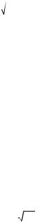
Let the target range track coordinate extrapolation for the next nth radar antenna scanning be carried out using the data of previous (n − 1)th radar antennas scanning. Position of the extrapolated point is denoted by O (see Figure 4.3). We think that the origin of Cartesian coordinate system is located at the point O. The axis Y is matched with “radar system–target” direction, the axis X is a perpendicular to the “radar system–target” direction away from radar antenna rotation, and the axis Z is directed in such way that we have a right-handed coordinate system. Then the random deviations x, y, z of the newly obtained under nth radar antenna scanning target pip from the gate center are defined in the following form:
|
xn = ±r ( |
βextrn |
+ |
βn ) |
|
|
|
|
|
|
|
|
yn = ± ( |
rnextr + |
rn ) |
(4.5) |
|
|
|||||
|
zn = ±r ( |
|
|
εn ) |
|
|
εextrn |
+ |
|
||
|
|
|
|
|
|
where
rnextr, Δβextrn , and Δεextrn are the random errors of coordinate extrapolation in the course of the nth
radar antenna scanning
rn, Δβn, and Δεn are the random errors of coordinate measuring in the course of the nth radar antenna scanning

120 Signal Processing in Radar Systems
|
et |
|
|
|
|
|
rg |
|
|
|
|
|
|
Ta |
trac |
|
|
|
|
|
|
|
|
3 |
|
|
|
|
|
1 |
|
|
|
|
|
k |
|
|
|
|
|
|
|
|
|
|
|
|
|
|
σy |
|
σζ |
0˝ |
ση |
|
σz |
|
|
|||
|
0 |
Y |
ζ |
|
η |
|
Radar-target |
|
|||||
|
|
σξ |
|
|
||
direction |
|
|
|
|
||
|
|
|
|
|
||
|
Z |
σx |
Vtg |
ξ |
|
|
|
|
|
|
|||
|
|
X |
σh |
|
2 |
|
|
|
|
0´ |
|
||
|
|
|
h |
|
|
|
|
|
|
|
σf |
|
|
|
|
|
σg |
|
|
|
|
|
|
|
f |
|
|
|
|
|
|
|
|
|
g
FIGURE 4.3 Extrapolation of target coordinates.
Under the definition of gate dimensions we can believe that the components rn, Δβn, and Δεn are statistically independent, do not depend on the scanning number step n, and are subjected to the normal Gaussian pdf with zero mean and variances σ2x, σ2y, and σ2z , respectively. Consequently, the joint pdf can be defined in the following form:
|
|
|
|
|
|
|
|
|
|
|
|
|
|
|
|
|
|
|
|
|
|
|
|
1 |
|
|
1 |
|
( |
x) |
2 |
|
( y) |
2 |
|
( z) |
2 |
|
|
|
|
f ( x, |
y, |
z) = |
|
|
|
exp − |
|
|
|
|
|
+ |
|
|
+ |
|
|
|
, |
(4.6) |
(2π)3 |
σ2x |
σ2yσ2z |
2 |
|
2 |
|
2 |
|
2 |
|
||||||||||
|
|
|
|
|
|
σ x |
|
|
σ y |
|
|
σz |
|
|
|
|
||||
|
|
|
|
|
|
|
|
|
|
|
|
|
|
|
|
|
|
|
|
|
and the surface corresponding to equal pdf is defined by the following equation:
( x)2 |
+ |
( |
y)2 |
+ |
( |
z)2 |
= λ2 , |
(4.7) |
σ2x |
|
σ2y |
|
σ2z |
||||
|
|
|
|
|
|
where λ is the arbitrary constant. Dividing the leftand right-hand side of (4.7) by λ2, we obtain
( x)2 |
+ |
( y)2 |
+ |
( z)2 |
= 1. |
(4.8) |
|
λ2σ2x |
λ2σ2y |
λ2σ2z |
|||||
|
|
|
|
Equation 4.8 is the ellipsoid equation with conjugate axles λσx, λσy, and λσz. At λ = 1, we obtain the unit ellipsoid—see ellipsoid 1 in Figure 4.3.
Henceforth, we believe that dynamical errors of extrapolation caused by contingency target maneuver are also normally distributed and have independent components on the F, G, and H axes. The F axis is matched with the target velocity vector; the G axis is directed in opposition to a tangential acceleration; and the H axis supplements the system to the right-handed coordinate one. Origin of the obtained coordinate system, as well as in the case of the previous coordinate system, coincides with the extrapolated point O. For better visualization the origin is replaced at the point O′ in Figure 4.3.
Algorithms of Target Range Track Detection and Tracking |
121 |
In 3D space the dynamic errors form an ellipsoid of equal probabilities, an equation of which takes the following form:
( f )2 |
|
( g)2 |
|
( h)2 |
|
(4.9) |
|
λ2σ2f |
+ λ2σ2g |
+ |
λ2σh2 = 1, |
||||
|
|||||||
the ellipsoid 2 in Figure 4.3 at λ = 1. If we add ellipsoids 1 and 2, then ellipsoid 3 will be formed, and directions of conjugate axles (the directions of axes of the Cartesian coordinate system Oηξζ with respect to the axes of the Cartesian coordinate system OXYZ and variances σ2η, σ2ξ, and σ2ζ by these axles) are defined by summing rules in space of independent vectorial deviations, caused by random and dynamic errors. For better visualization, the origin of the coordinate system Oηξζ is replaced at the point O″ in Figure 4.3.
The joint pdf of random components Δη, Δξ, and Δζ takes the following form:
p( η, ξ, |
ζ) = |
|
|
|
1 |
|
|
exp(−0.5λ |
2 |
), |
(4.10) |
||
(2π)3 σ2ησξ2σζ2 |
|
||||||||||||
|
|
|
|
|
|
|
|
|
|
|
|
|
|
where |
|
|
|
|
|
|
|
|
|
|
|
|
|
λ |
2 = |
( |
η)2 |
+ |
( |
ξ)2 |
+ |
( |
ζ)2 |
. |
|
|
(4.11) |
σ2η |
|
σξ2 |
|
|
|
|
|||||||
|
|
|
|
|
|
σζ2 |
|
|
|
||||
Thus, a surface of equally probable deviation of true target pips from the gate center represents an ellipsoid, value and direction of conjugate axles of which relative to the direction “radar system– target” depend on coordinate measurement errors, target maneuver intensity, and vectorial direction of target moving. Under ellipsoid distribution of true target pip deviation from the gate center, it is evident that the gate must have an ellipsoid shape with the conjugate axles λση, λσξ, and λσζ, where λ is the enlargement factor of the gate dimensions in comparison with the dimensions of unit ellipsoid to ensure the given before expectancy of hitting of true target pip within the gate.
The expectancy of random point hitting into the ellipsoid that is similar and has a similar disposition as ellipsoids of equal probabilities is defined in the following form:
|
|
|
1 |
|
|
|
|
P(λ) = 2 |
Φ0 |
(λ) − |
|
λ exp(−0.5λ2 ) |
, |
(4.12) |
|
2π |
|||||||
|
|
|
|
|
|
where Φ0(λ) is the standard normal Gaussian pdf given by (3.110). At λ ≥ 3, the probability P(λ) is very close to unit. There is a need to choose just the values of λ, forming an ellipsoid gate.
In practice, forming the ellipsoidal gates is impossible both under physical and mathematical gating. By this reason, the best thing that can be done is to form a gate in the shape of parallelepiped defined around the total error ellipsoid, as shown in Figure 4.3 (3). Parallelepiped side dimensions are equal to 2λση, 2λσξ, and 2λσζ, and its volume is defined as
Vpar = 8λ3σησξσζ . |
(4.13) |
Taking into consideration the fact that the volume of total error ellipsoid is defined as
Vel = |
4 |
πλ3σησξσζ , |
(4.14) |
|
3 |
||||
|
|
|
122 |
Signal Processing in Radar Systems |
βgate
εgate 
rgate
FIGURE 4.4 Definition of the simplest gate.
the gate volume is increased twice in comparison with the optimal volume. This phenomenon leads to an increase in the expectancy of hitting of false target pips within the gate or an increase in the number of target pips belonging to another target range tracks and, consequently, to deterioration of selection and resolution during gating operation.
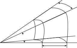
During the processing of high number of targets in real time by the computer subsystem of a complex radar system (CRS), computation of dimensions and orientation of parallelepiped gate sides is very cumbersome. In this case, there is a need to use a simple version of gating, a sense of which is the following. The simplest gate shape is chosen for definition in that coordinate system, in which radar information is processed. In the case of spherical coordinate system, the simplest gate is given by linear dimension in target range rgate and by two angular dimensions, namely, by the
azimuth Δβgate and elevation Δεgate (see Figure 4.4).
These dimensions can be preset based on maximal magnitudes of random and dynamic errors while processing all target range tracks. In short, in this case, the gate dimensions are chosen so that the ellipsoid of all possible (under all directions of target moving and flight) total deviations of true target pips from corresponding extrapolated points will be easily fit and rotated in any direction inside the gate. This is the crudest technique of gating. In conclusion, we note that all procedures, which are discussed in this subsection, to choose dimensions of 3D gate can be used in full during gating in plane for binding newly obtained target pips in 2D radar systems.
4.1.2 Algorithm of Target Pip Indication by Minimal Deviation from Gate Center
We consider a case of target pip indication under definition of target range track for a single target. At the same time, we assume that in addition to true target pips, the false target pips caused by noise and interferences passed over preprocessing filters can be present within the gate. Given the earlierprovided situation, the following varied decisions could be made:
•When there are several target pips, there is a need to continue to define the target range tracks using each target pip; in other words, we can suppose multiple target range tracks. Prolongation of target range tracks using false target pips will be canceled over several radar antennas scanning owing to absence of confirmations, but prolongation of the target range tracks using the true target pips will be continued. Such way of newly obtained target pip binding is very tedious. Moreover, when the density of false target pips is high, an avalanche-like increase in false target tracks leading to overload of memory devices in computer subsystems is possible.
•We must choose a single target pip within the gate, and we should be sure that the probability of the event that this target pip belongs to the target range tracking is the highest. Other target pips can be rejected as false. Such approach is appropriate with a view to decreasing the computation cost, but it requires a solution for the optimal target pip indication problem.