

Лекции_Микроэкономика
.pdfA.Friedman |
ICEF-2012 |
u
u c2
pu c1 1 p u c2 u pc1 1 p c2
u c1 |
|
|
|
|
0 |
c1 |
pc1 1 p c2 |
c2 |
c |
Application 1. Obtaining additional information
Mary has a utility function u=50-120/c, where c is her consumption, measured in thousands of dollars. If Mary becomes an economist, she will make 30 thousand per year for certain. If she becomes a pediatrician, she will make $60 thousand if there is a baby boom and $12 thousand otherwise. The probability of a baby boom is p=0.5.
|
boom |
30 u(30)=50-120/30=46 |
|
|
|
|
|
|
|
|
p= ½ |
|
|
|
economist |
no |
EU |
economist |
46 |
|
|
|||
|
p= ½ |
|
|
|
|
|
30 u(30)=50-120/30=46 |
|
|
|
boom |
60 u(60)=50-120/60=48 |
|
|
pediatrician |
p= ½ |
|
|
|
|
no |
EU pediatrician |
||
|
p= ½ |
12 u(12)=50-120/12=40 48 40 / 2 44 |
||
|
|
|||
By comparing utilities, we can |
find that Mary prefers |
to become an economist as |
||
EU economist 46 44 EU pediatrician . |
|
|
|
|
Now suppose a consulting firm has prepared demographic projections that indicate which event will occur. Will she purchase the projection at price of $6000?
|
|
economist |
24 |
|
|
|
|
|
|
|
|
|
||
boom |
|
|
|
|
|
|
|
|
|
|
|
|
|
|
p= ½ |
pediatrician |
54 |
|
|
|
|
|
|
|
|
|
|||
|
|
|
|
|
|
|
|
|
|
|
|
|
||
|
p= ½ |
|
|
|
|
|
|
|
|
|
|
|
|
|
|
|
economist |
24 |
|
|
|
|
|
|
|
|
|
||
bust |
|
|
|
|
|
|
|
|
|
|
|
|
|
|
|
|
pediatrician |
6120 |
|
|
|
|
|
|
|
|
|
||
|
projection |
|
|
|
|
120 |
|
65 |
|
|
||||
EU |
|
|
0.5 50 |
|
|
|
0.5 50 |
|
|
|
50 |
|
46 |
44 |
|
|
|
|
|
||||||||||
|
|
|
|
24 |
|
|
|
54 |
|
18 |
|
|
||
As the maximum utility achieved without demographic projection was only 44 Mary would be willing to purchase this projection.
41

A.Friedman |
ICEF-2012 |
Application 2. Insurance |
|
Consider risk averse individual with initial wealth w . With probability |
p she can incur |
losses of L , 0 L w . Individual is offered to purchase insurance with insurance premiumper unit of insurance.
Insurance is actuarially fair if EV $1 p $ 0 or p .
If p , then insurance is unfair. The case of unfair favourable insurance ( p ) is quite unrealistic as insurance company incurs loss under this price.
Thus we will consider only fair and unfavourable insurance.
Two states of the world: “loss” and “no loss”.
Two contingent commodities: cL - consumption in case of loss, cNL - consumption in case of no loss.
Denote by z the quantity of insurance and assume that over-insurance is not allowed (you cannot insure more than L), then
cL w L z zcNL w z
0 z L
If we solve this system with respect to z , then we get the budget constraint of the form:
cNL |
w |
|
|
w L cL |
|
where w L cL |
w L . |
|||
|
|
|||||||||
|
|
|||||||||
|
1 |
|
|
|
|
|
|
|
||
The slope of budget line is / 1 . |
|
|
|
|
|
|
||||
|
|
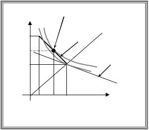
cNL |
endowment |
|
|
|
|
|
|
|
|
|
|
|
|
|
|
|
cL cNL |
|
|
|
|
|
|
|
|
|
||||
|
w |
|
|
|
|
|
||||
|
|
|
1 |
|
|
|||||
|
|
|
|
|
|
|
||||
|
|
|
|
budget line |
|
|
||||
w-L cL
The slope of fair odds line equals |
p |
|
|
. |
|
1 p |
||
In case of fair insurance budget constraint coincide with fair odds line and as a result utility is maximised at certainty point, where indifference curve is tangent to budget line, which means
that person will purchase full insurance: cL w L z 1 cNL w z or z L .
42

A.Friedman |
|
|
|
|
|
|
ICEF-2012 |
|
cNL |
cL |
cNL |
|
|
||
w |
|
|
|
||||
|
|
|
|
|
|
|
|
|
|
Optimal choice |
|
|
|
|
|
|
|
|
|
|
|
p |
|
|
|
|
|
|
|||
w L |
|
1 |
1 p |
||||
w L |
cL |
w L |
|
|
Fair insurance |
Thus any risk averse agent under fair insurance purchases full insurance (insures all the loss).
In case of unfair unfavourable insurance ( p ) budget line is steeper than fair odds line. As a result risk averse person will never purchase full insurance. He will either purchase partial insurance ( 0 z L ) or no insurance at all.
|
Optimal choice |
|
|
|
Optimal choice |
|
|
|
|
||||
cNL |
|
|
|
cL cNL |
|
cNL |
|
cL cNL |
|||||
w |
|
|
|
w |
|
|
|
||||||
|
|
|
|
|
|
|
|
|
|
||||
|
1 |
|
|
|
1 |
|
|
|
|
||||
w z |
|
|
|
|
|
|
|
|
|
|
|
p |
|
|
|
|
|
|
p |
|
|
|
|
|
|
||
|
|
|
|
|
|
|
|
|
|
|
|
||
|
|
|
|
|
|
|
|
|
|
p |
|||
|
|
|
|
|
|
|
|
|
|
1 |
|||
|
|
|
|
1 p |
|
|
|
|
|||||
|
|
|
|
|
|
|
|
|
|
|
|
||
cL |
cL |
w L |
w L |
Unfavourable insurance
Application 3. Diversification
Consider a risk averse investor with initial wealth, w than he can allocate between two assets. One asset is risk-free with net return equal zero. The other asset is risky. In bad state of the world net return is 1 b 0 and in good state net return is a 0 . The probability of good state is p . Suppose that on average risky project gives higher return bp a 1 p 0 .
Two states of the world: “bad” and “good”.
Two contingent commodities: c1 - consumption in case of bad state, c2 - consumption in case of good state.
Denote by z investment in risky asset (assume 0 z w ), then
43
A.Friedman |
|
|
|
|
|
|
|
|
|
|
ICEF-2012 |
|
|
c1 w z 1 b z w bz |
|
||||||||
|
|
c |
w z 1 a z w az |
|
|||||||
|
|
|
2 |
|
|
|
|
|
|
|
|
|
|
|
|
|
|
|
|
|
|
|
|
|
|
0 z w |
|
|
|
|
|
|
|||
If we solve this system with respect to z , then we get the budget constraint of the form: |
|||||||||||
c |
|
w |
b |
w c where |
w 1 b c w . |
||||||
2 |
|
||||||||||
|
|
a |
1 |
|
|
|
|
|
|
1 |
|
|
|
|
|
|
|
|
|
|
|
|
|
The slope of budget line is a / b . |
|
|
|
|
|
|
|
|
|
||
The absolute value of the slope of fair odds line is |
|
p |
|
a |
|
as bp a 1 p 0 . |
|||||
|
p |
|
|||||||||
|
|
|
|
1 |
|
|
b |
|
|||
|
|
c2 |
|
Optimal choice |
|
|
|
|
|
|
|
|
|
|
|
|
|
|
|
|
|
|
|
|
|
|
|
|
|
cL cNL |
|
||||
|
w 1 a |
|
a / b |
|
|
|
|
|
|
||
|
|
|
|
|
|
|
|
|
p |
|
|
|
|
|
|
|
|
|
|
|
|||
|
|
w |
|
|
|
|
1 p |
|
|||
|
|
|
|
|
|
|
|
|
|
|
|
|
|
w 1 b w |
|
c1 |
|
||||||
|
|
|
|
|
|
|
|
||||
|
|
|
|
Diversification |
|
|
|
|
|
|
|
Conclusion: if risk is favourable, then risk averse agent will invest positive sum in risky asset (i.e. he will diversify).
44

A.Friedman |
ICEF-2012 |
4. THE FIRM
4.1 Modeling the firm’s technological opportunities
Production function is the relationship between the quantities of various inputs used per period of time and the maximum quantity of output that can be produced per period of time:
Q f z1 ,z2 , ,zn .
We are going to concentrate on the case with two inputs: capital (K) and labour (L). Examples of production functions ( 0, 0 ):
Fixed proportions or Leontieff technology min L, K ,
Linear technology L K ,
Cobb-Douglas production function AL K
In case of two inputs we can represent production function graphically in terms of isoquants.
Isoquant is the locus of all the (technically efficient) combinations of inputs for producing a given level of output.
Question: illustrate isoquants for the Leontieff, linear and Cobb-Douglas production functions.
Properties of the production functions.
Marginal physical product of input i - the extra amount of output that can be produced when the firm uses additional unit of this input, holding the levels of other inputs constant:
MPi f .zi
A technology exhibits decreasing/increasing/constant returns to factor when the marginal physical product of an input falls/rises/stays constant as the amount of the input used increases.
Question: characterize the three considered technologies (Leontieff, linear and CobbDouglas) with respect to returns to each factor of production
Marginal rate of technical substitution of labour for capital MRTSLK measures the rate at which the firm has to substitute one input (L) for another (K) in order to keep output (Q)
constant: MRTS |
|
|
dK |
|
|
|
. Thus MRTS equals to the absolute value of the slope of an |
|
LK |
dL |
|||||||
|
|
|
|
|
||||
isoquant. |
|
|
|
Q const |
|
|||
|
|
|
|
|||||
|
|
|
|
|
|
|
||
Definition suggests that MRTS can be calculated as a ratio of the marginal products:
dQ f dK f |
dL 0 |
, which implies MRTS |
|
|
dK |
|
|
|
|
f L |
|
MPL |
. |
||
|
|
|
|
||||||||||||
LK |
|
|
|
|
|
|
|||||||||
K |
|
L |
|
|
dL |
|
|
|
|
f |
|
|
MP |
||
|
|
|
|
|
|
|
Q const |
|
|
|
|||||
If MRTSLK |
|
|
|
|
|
|
|
|
|
|
K |
|
K |
||
is |
some |
positive constant, then |
the factors |
are |
|
perfect substitutes (linear |
|||||||||
technology) |
|
|
|
|
|
|
|
|
|
|
|
|
|
|
|
|
|
|
|
|
|
|
|
|
|
|
|
|
45 |
||

A.Friedman |
ICEF-2012 |
If MRTSLK is 0, then the factors are perfect complements (Leontieff. Note: MRTS is not defined at kink)
If MRTSLK isn’t constant, then the factors are imperfect substitutes (Cobb-Douglas).
In case of Cobb-Douglas technology we observe diminishing MRTS while moving along the isoquant.
Most |
of the |
production functions used in |
K |
empirical analyses are homothetic functions. |
|
||
(Note: function |
f is homothetic if f h g z , |
|
|
where |
g z is homogeneous of degree 1 and |
|
|
h is monotone). For homothetic production
functions the slopes of the isoquants are preserved along every ray through the origin, i.e. MRTS remains the same for any given K/L ratio whatever the level of output.
0
Returns to scale
Q2
Q1
L
If all inputs are changed by the same proportion this is referred to as a change in the scale of production.
Decreasing returns to scale (DRS): a proportional increase in all inputs leads to less than proportionate increase in output: f L, K f L,K for all L,K and 1.
Constant returns to scale (CRS): a proportional increase in all inputs leads to proportionate increase in output: f L, K f L,K for all L,K and 0 .
Increasing returns to scale (IRS): a proportional increase in all inputs leads to greater than proportionate increase in output: f L, K f L,K for all L,K and 1.
Returns to scale for homogenous production functions
Note: production function is homogeneous of degree t if f L, K t f L,K for allL,K and 0 .
If t 1, then we have CRS technology, If t 1, then we have IRS technology, If t 1, then we have DRS technology.
4.2 Profit maximization and Cost minimisation
Profit maximization problem
max pQ wL rK
K 0,L 0
f K ,L Q
46

A.Friedman |
ICEF-2012 |
Solution: demand functions for factors of production L p,w,r , K p,w,r and supply of output Q p,w,r
This problem can be divided into 2 sub-problems:
TC w,r ,Q |
min wL rK |
|
1) Cost minimization problem |
K 0,L 0 |
|
|
|
|
|
f K ,L Q |
|
Solution: conditional demand functions for factors of production L w,r,Q , |
K w,r,Q , |
|
TC w,r,Q wL w,r,Q rK w,r,Q -cost function |
|
|
2) profit maximization with respect to output max pQ TC w,r,Q .
Q 0
4.3 Cost minimization
Cost minimization in the long run
In the long-run all factors are variable
TC LR w,r,Q min wL rK
K 0,L 0
F K ,L Q
Graphical solution of cost-minimisation problem
K
K |
isocost lines |
|
|
|
Q1 |
0 |
L |
L |
|
|
Isocost line - a line representing all input combinations that have the same cost for the firm. Equation of isocost: wL rK const
At interior solution the slope of isoquant is equal to the slope of isocost:
MRTSLK L ,K w / r . This condition implies that if the firm uses both factors in equilibrium, then they bring the same marginal product per dollar spent:
MP |
L ,K |
|
MP |
L ,K |
. |
||
L |
|
|
K |
|
|
||
|
|
|
|
|
|
||
|
w |
|
|
r |
|
||
Thus if the firm uses both factors, then the corresponding quantities demanded can be found from the following system
F L ,K Q |
||
|
|
|
|
|
L ,K w / r |
MRTS |
LK |
|
|
|
|
47

A.Friedman |
ICEF-2012 |
Let L w,r,Q and |
K w,r,Q be the solutions of long run cost minimization problem. These |
demand functions are called conditional or derived demand for factors of production since the quantities depend on the level of output produced.
We can look for the optimum input combinations in production for different levels of output, the resulting curve is known as expansion path. Expansion path allows for given factor prices to get a relationship between output and the long run cost.
K
Expansion
path
Q4
Q3
Q1 Q2
0 |
L |
Exercise. Illustrate expansion path for the homothetic production function.
Analytically we get he long run cost function by plugging conditional demand functions into the objective function: TC LR w,r,Q wL w,r,Q rK w,r,Q .
Properties of long run costs
Long run marginal cost ( MC LR ) - the change in long-run total cost due to the production of
additional unit of output: MC LR TC LR .Q
Long run average cost ( AC LR ) - the long-run total cost divided by the number of unites
produced: AC LR TC LR .
Q
When long run average costs fall as output rises, costs are said to exhibit economies of scale.
When long run average costs rise with the output level, costs are said to exhibit diseconomies of scale.
Due to homotheticity, K/L ratio under CRS is not affected by the level of output. As a result, with CRS technology to increase output in times we increase the employment of each factor in times. Then cost of production also increases in times, while average cost stay constant:
AC LR Q |
TC LR Q |
|
|
TC LR Q |
|
TC LR Q |
|
AC LR Q . |
|
Q |
Q |
Q |
|||||||
|
|
|
|
||||||
That is in case of CRS we have neither economies, nor diseconomies of scale.
NOTE: As AC=const, then TC LR cQ , where c - cost of producing of one unit of output. It
implies that AC LR MC LR c .
48

A.Friedman |
ICEF-2012 |
AC |
CRS technology |
0 |
Q |
|
With IRS we can produce Q by increasing the factors’ employment in a smaller proportion,
which implies that total cost also increase by less than times1. As a result AC falls and we deal with economies of scale:
AC LR Q |
TC LR Q |
|
|
TC LR Q |
|
TC LR Q |
|
AC LR Q . |
|
Q |
Q |
Q |
|||||||
|
|
|
|
||||||
|
AC |
IRS technology |
|
|
|
|
|||
0 |
Q |
|
In case of DRS under homothetic production function in order to increase output in times, we increase the factors’ employment in a greater proportion, which implies that total cost also increases in more than times. As a result AC goes up:
AC LR Q |
TC LR Q |
|
|
TC LR Q |
|
TC LR Q |
|
AC LR Q . |
|
Q |
Q |
Q |
|||||||
|
|
|
|
||||||
|
AC |
DRS technology |
|
|
|
|
|||
0 |
Q |
|
That is in case of DRS we have diseconomies of scale.
Relationships between LRAC and LRMC |
|
|
|
|
|
|
|
|
If TC(0)=0, then AC 0 MC 0 . Proof: AC 0 lim |
TC Q |
|
lim |
MC Q |
MC 0 . |
|
Q |
|
1 |
|
||||
|
Q 0 |
Q 0 |
|
|
|||
1 Note if production function isn’t homothetic then proportional factor increase does not necessarily correspond to cost minimizing bundle but this implies that cost minimizing bundle might cost even less.
49

A.Friedman |
|
|
|
|
|
|
|
|
|
|
|
|
|
|
|
|
ICEF-2012 |
If AC reaches minimum at Q 0, then |
AC Q MC Q , |
|
|||||||||||||||
Proof. If |
|
AC |
reaches |
minimum at |
Q 0, then |
AC Q 0 , which implies |
|||||||||||
AC Q |
TC Q |
|
Q |
TC Q TC Q |
|
|
MC Q AC Q |
|
or AC Q MC Q . |
||||||||
|
|
|
|
||||||||||||||
|
|
|
|
|
|
|
|
|
|
|
|
|
|
|
0 |
||
|
|
|
|
2 |
|
|
|
2 |
|
|
|||||||
|
|
Q |
|
|
|
|
Q |
|
|
|
Q |
|
|
|
|
||
|
|
|
|
|
|
|
|
|
|
|
|
|
|
|
|||
If AC diminishes over some range of outputs, then |
AC Q MC Q for all Q from |
||||||||||||||||
considered range, |
|
|
|
|
|
|
|
|
|
|
|
|
|||||
Proof. If AC diminishes over some range of Q , then AC Q 0 for each Q from given
range. This implies that
or AC Q MC Q .
TC Q |
|
||
|
|||
AC Q |
|
|
|
|
|
||
|
Q |
|
|
|
|
|
|
|
Q TC Q TC Q |
|
MC Q AC Q |
0 |
|||
Q2 |
|
Q2 |
|
||||
|
|
|
|||||
If AC increases over some range of outputs, then AC Q MC Q for all Q from considered range.
Proof. If AC increases over some range of Q , then AC Q 0 for each Q from given
range. This implies that
or AC Q MC Q .
TC Q |
|
||
|
|||
AC Q |
|
|
|
|
|
||
|
Q |
|
|
|
|
|
|
|
Q TC Q TC Q |
|
MC Q AC Q |
0 |
|||
Q2 |
|
Q2 |
|
||||
|
|
|
|||||
Exercise. Suppose that AC and MC are U-shaped and TC(0)=0. Sketch AC and MC curves on the same graph.
Cost minimization in the short-run
In the short-run capital is fixed and we choose only one variable factor - labour:
TC SR w,r,Q,K min wL rK
|
|
|
|
|
L 0 |
|
|
|
|
|
|
|
|
|||
|
|
|
|
F |
|
,L Q |
|
|
|
|
|
|
|
|
||
K |
|
|
|
|
|
|
|
|
||||||||
If F |
|
,0 0 , then labour employment is given by the condition |
F |
|
,L Q . Solving this |
|||||||||||
K |
K |
|||||||||||||||
equation, we get short run demand for labour L L Q, |
|
|
. Plugging into the objective |
|||||||||||||
K |
||||||||||||||||
function we get short-run total cost as a sum of variable cost (VC) and fixed cost (FC): |
||||||||||||||||
|
|
TC SR w,r,Q, |
|
wL Q, |
|
|
|
|
|
|
|
|
||||
|
|
K |
K |
rK . |
|
|
|
|||||||||
|
|
|
|
|
|
|
|
|
||||||||
|
|
|
|
fixed cost |
|
|
|
|||||||||
|
|
|
|
var iable cost |
|
|
|
|
|
|
|
|
||||
At interior solution the slope of isoquant is equal to the slope of isocost:
Properties of the short-run cost
Short-run marginal cost ( MC SR ) - the change in short-run total cost due to the production of
additional unit of output: MC SR TC SR .Q
50