Вопрос 7 Structure of the Human Auditory System

A simplified diagram of the human auditory system appears in Figure 1.13. The pinna (or informally the ear) is the surface surrounding the canal in which sound is funneled. Sound waves are guided by the canal toward the eardrum—a mem- brane that acts as an acoustic-to-mechanic transducer. The sound waves are then translated into mechanical vibrations that are passed to the cochlea through a series of bones known as the ossicles. Presence of the ossicles improves sound propaga- tion by reducing the amount of reflection and is accomplished by the principle of impedance matching.

The cochlea is a rigid snail-shaped organ filled with fluid. Mechanical oscilla- tions impinging on the ossicles cause an internal membrane, known as the basilar membrane, to vibrate at various frequencies. The basilar membrane is characterized by a set of frequency responses at different points along the membrane; and a sim- ple modeling technique is to use a bank of filters to describe its behavior. Motion along the basilar membrane is sensed by the inner hair cells and causes neural activities that are transmitted to the brain through the auditory nerve.

The different points along the basilar membrane react differently depending on the frequencies of the incoming sound waves. Thus, hair cells located at different positions along the membrane are excited by sounds of different frequencies. The neurons that contact the hair cells and transmit the excitation to higher auditory centers maintain the frequency specificity. Due to this arrangement, the human auditory system behaves very much like a frequency analyzer; and system characterization is simpler if done in the frequency domain.

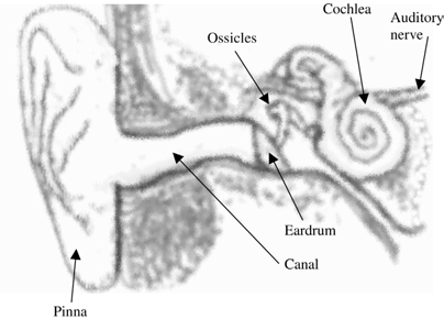
Figure 1.13 Diagram of the human auditory system.

200

AT( f ) ¹⁰⁰

0

3 4 5

10 100 1 ^10

f

1 ^10

1 ^10

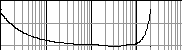
Figure 1.14 A typical absolute threshold curve.

Вопрос 8 Absolute Threshold

The absolute threshold of a sound is the minimum detectable level of that sound in the absence of any other external sounds. That is, it characterizes the amount of energy needed in a pure tone such that it can be detected by a listener in a noiseless environment. Figure 1.14 shows a typical absolute threshold curve, where the hor- izontal axis is frequency measured in hertz (Hz); while the vertical axis is the abso- lute threshold in decibels (dB), related to a reference intensity of 10^—12 watts per square meter—a standard quantity for sound intensity measurement.

Note that the absolute threshold curve, as shown in Figure 1.14, reflects only the average behavior; the actual shape varies from person to person and is measured by presenting a tone of a certain frequency to a subject, with the intensity being tuned until the subject no longer perceive its presence. By repeating the measurements using a large number of frequency values, the absolute threshold curve results.

As we can see, human beings tend to be more sensitive toward frequencies in the range of 1 to 4 kHz, while thresholds increase rapidly at very high and very low frequencies. It is commonly accepted that below 20 Hz and above 20 kHz, the auditory system is essentially dysfunctional. These characteristics are due to the structures of the human auditory system: acoustic selectivity of the pinna and canal, mechanical properties of the eardrum and ossicles, elasticity of the basilar membrane, and so on.

We can take advantage of the absolute threshold curve in speech coder design.

Some approaches are the following:

• Any signal with an intensity below the absolute threshold need not be considered, since it does not have any impact on the finalquality of the coder.

• More resources should be allocated for the representation of signals within the most sensitive frequency range, roughly from 1 to 4 kHz, since distortions in this range are more noticeable.

Masking

Masking refers to the phenomenon where one sound is rendered inaudible because of the presence of other sounds. The presence of a single tone, for instance, can

Power

Frequency

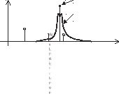
Figure 1.15 Example of the masking curve associated with a single tone. Based on the masking curve, examples of audible (&) and inaudible (*) tones are shown, which depend on whether the power is above or below the masking curve, respectively.

mask the neighboring signals—with the masking capability inversely proportional to the absolute difference in frequency. Figure 1.15 shows an example where a sin- gle tone is present; the tone generates a masking curve that causes any signal with power below it to become imperceptible. In general, masking capability increases with the intensity of the reference signal, or the single tone in this case.

The features of the masking curve depend on each individual and can be mea- sured in practice by putting a subject in a laboratory environment and asking for his/her perception of a certain sound tuned to some amplitude and frequency values in the presence of a reference tone.

Masking can be explored for speech coding developments. For instance, analyz- ing the spectral contents of a signal, it is possible to locate the frequency regions that are most susceptible to distortion. An example is shown in Figure 1.16. In this case a typical spectrum is shown, which consists of a series of high- and low-power regions, referred to as peaks and valleys, respectively. An associated masking curve exists that follows the ups and downs of the original spectrum. Signals with power below the masking curve are inaudible; thus, in general, peaks can tolerate more distortion or noise than valleys.

Power

Frequency

Figure 1.16 Example of a signal spectrum and the associated masking curve. Dark areas correspond to regions with relatively little tolerance to distortion, while clear areas correspond to regions with relatively high tolerance to distortion.

A well-designed coding scheme should ensure that the valleys are well preserved or relatively free of distortions; while the peaks can tolerate a higher amount of noise. By following this principle, effectiveness of the coding algorithm is improved, leading to enhanced output quality.

As we will see in Chapter 11, coders obeying the principle of code-excited linear prediction (CELP) rely on the perceptual weighting filter to weight the error spec- trum during encoding; frequency response of the filter istime-varying and depends on the original spectrum of the input signal. The mechanism is highly efficient and is widely applied in practice.

Phase Perception

Modern speech coding technologies rely heavily on the application of perceptual characteristics of the human auditory system in various aspects of a quantizer’s design and general architecture. In most cases, however, the focus on perception is largely confined to the magnitude information of the signal; the phase counterpart has mostly been neglected with the underlying assumption that human beings are phase deaf.

There is abundant evidenceon phase deafness; for instance, a single tone and its time-shifted version essentially produce the same sensation; on the other hand, noise perception is chiefly determined by the magnitude spectrum. This latter example was already described in the last section for the design of a rudimentary coder and is the foundation of some early speech coders, such as the linear predic- tion coding (LPC) algorithm, studied in Chapter 9.

Even though phase has a minor role in perception, some level of phase preserva- tion in the coding process is still desirable, since naturalness is normally increased. The code-excited linear prediction (CELP) algorithm, for instance, has a mechanism to retain phase information of the signal, covered in Chapter 11.