

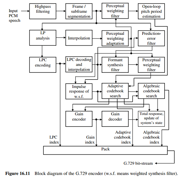
24/25 Speech encoding. Acelp (g.729) coder
ALGEBRAIC CELP or ACELP was born as another attempt to reduce the computational cost of standard CELP coders. As explained in Chapter 11, excitation codebook search is the most intensive of all CELP operations. Throughout history,
researchers have tried many techniques to bring the cost down to manageable
levels; very often, the approach is to impose a certain structure for the fixed excitation codebook so as to enable fast search methods.
Summary of Decoding Operations
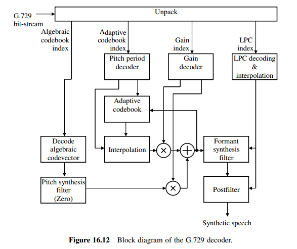
Figure 16.12 shows the decoder. The algebraic codevector is found from the received index, specifying positions and signs of the four pulses, which is filtered by the pitch synthesis filter in zero state. Parameters of this filter are specified in Section 16.4. The adaptive codevector is recovered from the integer part of the pitch period and interpolated according to the fractional part of the pitch period. Algebraic and adaptive codevectors are scaled by the decoded gains and added to form
the excitation for the formant synthesis filter. A postfilter is incorporated to improve subjective quality.
26iLBC
Encoder
The input to the encoder SHOULD be 16 bit uniform PCM sampled at 8
kHz. It SHOULD be partitioned into blocks of BLOCKL=160/240 samples
for the 20/30 ms frame size. Each block is divided into NSUB=4/6
consecutive sub-blocks of SUBL=40 samples each. For 30 ms frame
size, the encoder performs two LPC_FILTERORDER=10 linear-predictive
coding (LPC) analyses. The first analysis applies a smooth window
centered over the second sub-block and extending to the middle of the
fifth sub-block. The second LPC analysis applies a smooth asymmetric
window centered over the fifth sub-block and extending to the end of
the sixth sub-block. For 20 ms frame size, one LPC_FILTERORDER=10
linear-predictive coding (LPC) analysis is performed with a smooth
window centered over the third sub-frame.
For each of the LPC analyses, a set of line-spectral frequencies
(LSFs) are obtained, quantized, and interpolated to obtain LSF
coefficients for each sub-block. Subsequently, the LPC residual is
computed by using the quantized and interpolated LPC analysis
filters.
The two consecutive sub-blocks of the residual exhibiting the maximal
weighted energy are identified. Within these two sub-blocks, the
start state (segment) is selected from two choices: the first 57/58
samples or the last 57/58 samples of the two consecutive sub-blocks.
The selected segment is the one of higher energy. The start state is
encoded with scalar quantization.
A dynamic codebook encoding procedure is used to encode 1) the 23/22
(20 ms/30 ms) remaining samples in the two sub-blocks containing the
start state; 2) the sub-blocks after the start state in time; and 3)
the sub-blocks before the start state in time. Thus, the encoding
target can be either the 23/22 samples remaining of the two sub-
blocks containing the start state or a 40-sample sub-block. This
target can consist of samples indexed forward in time or backward in
time, depending on the location of the start state.
The codebook coding is based on an adaptive codebook built from a
codebook memory that contains decoded LPC excitation samples from the
already encoded part of the block. These samples are indexed in the
same time direction as the target vector, ending at the sample
instant prior to the first sample instant represented in the target
vector. The codebook is used in CB_NSTAGES=3 stages in a successive
refinement approach, and the resulting three code vector gains are
encoded with 5-, 4-, and 3-bit scalar quantization, respectively.
The codebook search method employs noise shaping derived from the LPC
filters, and the main decision criterion is to minimize the squared
error between the target vector and the code vectors. Each code
vector in this codebook comes from one of CB_EXPAND=2 codebook
sections. The first section is filled with delayed, already encoded
residual vectors. The code vectors of the second codebook section
are constructed by predefined linear combinations of vectors in the
first section of the codebook.
As codebook encoding with squared-error matching is known to produce
a coded signal of less power than does the scalar quantized start
state signal, a gain re-scaling method is implemented by a refined
search for a better set of codebook gains in terms of power matching
after encoding. This is done by searching for a higher value of the
gain factor for the first stage codebook, as the subsequent stage
codebook gains are scaled by the first stage gain.
28. Decoder
Typically for packet communications, a jitter buffer placed at the
receiving end decides whether the packet containing an encoded signal
block has been received or lost. This logic is not part of the codec
described here. For each encoded signal block received the decoder
performs a decoding. For each lost signal block, the decoder
performs a PLC operation.
The decoding for each block starts by decoding and interpolating the
LPC coefficients. Subsequently the start state is decoded.
For codebook-encoded segments, each segment is decoded by
constructing the three code vectors given by the received codebook
indices in the same way that the code vectors were constructed in the
encoder. The three gain factors are also decoded and the resulting
decoded signal is given by the sum of the three codebook vectors
scaled with respective gain.
An enhancement algorithm is applied to the reconstructed excitation
signal. This enhancement augments the periodicity of voiced speech
regions. The enhancement is optimized under the constraint that the
modification signal (defined as the difference between the enhanced
excitation and the excitation signal prior to enhancement) has a
short-time energy that does not exceed a preset fraction of the
short-time energy of the excitation signal prior to enhancement.
A packet loss concealment (PLC) operation is easily embedded in the
decoder. The PLC operation can, e.g., be based on repeating LPC
filters and obtaining the LPC residual signal by using a long-term
prediction estimate from previous residual blocks.
3. Encoder Principles
The following block diagram is an overview of all the components of
the iLBC encoding procedure. The description of the blocks contains
references to the section where that particular procedure is further
described.
+-----------+ +---------+ +---------+
speech -> | 1. Pre P | -> | 2. LPC | -> | 3. Ana | ->
+-----------+ +---------+ +---------+
+---------------+ +--------------+
-> | 4. Start Sel | ->| 5. Scalar Qu | ->
+---------------+ +--------------+
+--------------+ +---------------+
-> |6. CB Search | -> | 7. Packetize | -> payload
| +--------------+ | +---------------+
----<---------<------
sub-frame 0..2/4 (20 ms/30 ms)
Figure 3.1. Flow chart of the iLBC encoder
1. Pre-process speech with a HP filter, if needed (section 3.1).
2. Compute LPC parameters, quantize, and interpolate (section 3.2).
3. Use analysis filters on speech to compute residual (section 3.3).
4. Select position of 57/58-sample start state (section 3.5).
5. Quantize the 57/58-sample start state with scalar quantization
(section 3.5).
6. Search the codebook for each sub-frame. Start with 23/22 sample
block, then encode sub-blocks forward in time, and then encode
sub-blocks backward in time. For each block, the steps in Figure
3.4 are performed (section 3.6).
7. Packetize the bits into the payload specified in Table 3.2.
The input to the encoder SHOULD be 16-bit uniform PCM sampled at 8
kHz. Also it SHOULD be partitioned into blocks of BLOCKL=160/240
samples. Each block input to the encoder is divided into NSUB=4/6
consecutive sub-blocks of SUBL=40 samples each.
0 39 79 119 159
+---------------------------------------+
| 1 | 2 | 3 | 4 |
+---------------------------------------+
20 ms frame
0 39 79 119 159 199 239
+-----------------------------------------------------------+
| 1 | 2 | 3 | 4 | 5 | 6 |
+-----------------------------------------------------------+
30 ms frame
Figure 3.2. One input block to the encoder for 20 ms (with four sub-
frames) and 30 ms (with six sub-frames).
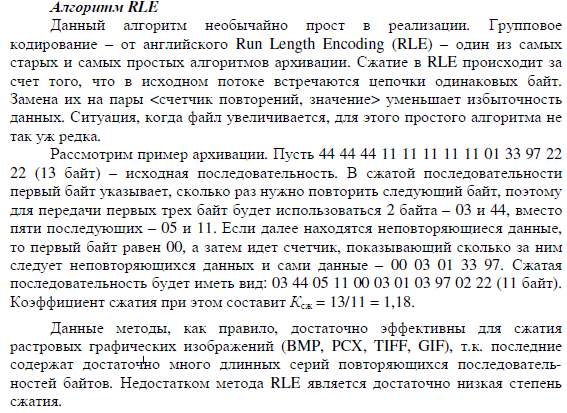
Lossless data compression algorithms. RLE
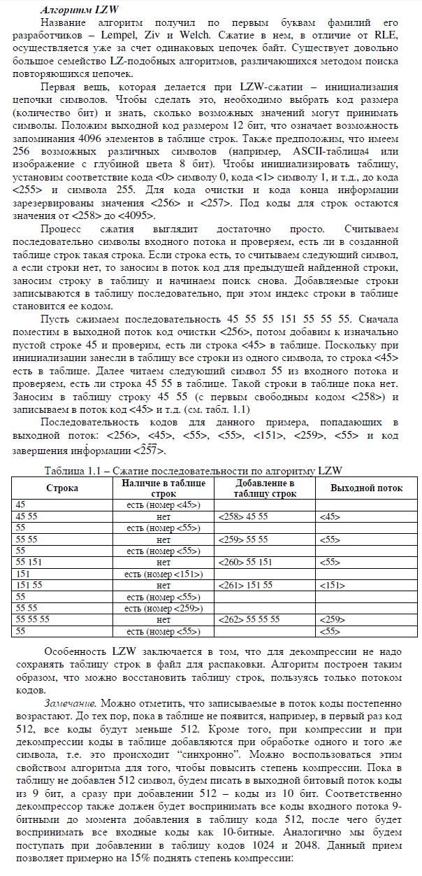
30. Lossless data compression algorithms. LZW
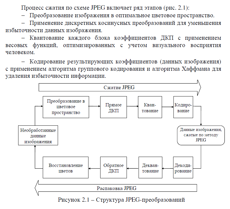
32. Image compression. JPEG
33. JPEG 2000 is an image compression standard and coding system. It was created by the Joint Photographic Experts Group committee in 2000 with the intention of superseding their original discrete cosine transform-based JPEG standard (created in 1992) with a newly designed, wavelet-based method. The standardized filename extension is .jp2 for ISO/IEC 15444-1 conforming files and .jpx for the extended part-2 specifications, published as ISO/IEC 15444-2. The registered MIME types are defined in RFC 3745. For ISO/IEC 15444-1 it is image/jp2.
Technical discussion:The aim of JPEG 2000 is not only improving compression performance over JPEG but also adding (or improving) features such as scalability and editability. JPEG 2000's improvement in compression performance relative to the original JPEG standard is actually rather modest and should not ordinarily be the primary consideration for evaluating the design. Very low and very high compression rates are supported in JPEG 2000. The ability of the design to handle a very large range of effective bit rates is one of the strengths of JPEG 2000. For example, to reduce the number of bits for a picture below a certain amount, the advisable thing to do with the first JPEG standard is to reduce the resolution of the input image before encoding it. That is unnecessary when using JPEG 2000, because JPEG 2000 already does this automatically through its multiresolution decomposition structure. The following sections describe the algorithm of JPEG 2000.
Performance, JPEG 2000 delivers a typical compression gain in the range of 20%, depending on the image characteristics. Higher-resolution images tend to benefit more, where JPEG-2000's spatial-redundancy prediction can contribute more to the compression process. In very low-bitrate applications, studies have shown JPEG 2000 to be outperformed[21] by the intra-frame coding mode of H.264. Good applications for JPEG 2000 are large images, images with low-contrast edges — e.g., medical images.
34. Digital video. Principles of video compression
Digital video is a type of digital recording system that works by using a digital rather than an analog video signal. Overview of basic properties[edit]
Digital video comprises a series of orthogonal bitmap digital images displayed in rapid succession at a constant rate. In the context of video these images are called frames.[2] We measure the rate at which frames are displayed in frames per second (FPS)Since every frame is an orthogonal bitmap digital image it comprises a raster of pixels. If it has a width of W pixels and a height of H pixels we say that the frame size is WxH.Pixels have only one property, their color. The color of a pixel is represented by a fixed number of bits. The more bits the more subtle variations of colors can be reproduced. This is called thecolor depth (CD) of the video.An example video can have a duration (T) of 1 hour (3600sec), a frame size of 640x480 (WxH) at a color depth of 24bits and a frame rate of 25fps. This example video has the following properties:
pixels per frame = 640 * 480 = 307,200
bits per frame = 307,200 * 24 = 7,372,800 = 7.37Mbits
bit rate (BR) = 7.37 * 25 = 184.25Mbits/sec
video size (VS)[3] = 184Mbits/sec * 3600sec = 662,400Mbits = 82,800Mbytes = 82.8Gbytes
The most important properties are bit rate and video size.