Добавил:

Upload Опубликованный материал нарушает ваши авторские права? Сообщите нам.

Вуз:

Одесская национальная академия связи им. А.С. Попова

Предмет:

[НЕСОРТИРОВАННОЕ]

Файл:

Functions of several variables- Textbook..pdf

.pdf

Скачиваний:

Добавлен:

10.02.2016

Размер:

1.51 Mб

Скачать

☆

1 / 51 2 3 4 5 > Следующая >>>

MINISTRY OF EDUCATION AND SCIENCE YOUTH AND SPORTS OF UKRAINE

ODESSA NATIONAL A.S.POPOV ACADEMY OF TELECOMMUNICATIONS

Department of Higher Mathematics

Gavdzinski V.N., Korobova L.N., Maltseva E.V.

FUNCTIONS OF SEVERAL VARIABLES

Textbook

Odessa – 2012

УДК 510(083)

План НМВ 2011/2012 уч.г.

Составители:

Доц. В. Н. Гавдзинский, ст. преп. Л. Н. Коробова, ст. преп. Е. В. Мальцева

Методическое пособие содержит основные определения, формулы и теоремы дифференциального исчисления функции многих переменных и предназначено для студентов академии, изучающих математику на английском языке.

Основные теоремы и формулы приведены с доказательством, а также даны решения типовых задач, задания для самостоятельной работы. Кроме того прилагаются комплексной контрольной работы.

	CONTENTS
1.	Definitions ..........................................................................................................	4
2.	Ways of representation functions of two variables .............................................	5
3.	Level curves .......................................................................................................	6
4.	Limits and continuity............................................................................................	8
5.	Partial increments and derivatives of the first order ...........................................	10
6.	Geometric interpretation of partial derivatives ...................................................	12
7.	Level surfaces. Quadric surfaces .........................................................................	13
8.	Tangent plane and normal ...................................................................................	15
9.	Total increment and total differential of a function of two variables ..................	16

10.	Applying a total differential to approximate calculations..................................	17
11.	Partial derivatives of the higher order ..............................................................	18
12.	Differentiating composite functions ..................................................................	19
13.	Directional derivative and gradient of a function of several variables .............	20
14.	Extreme of a function of two variables .............................................................	22
15.	The conditional extreme of a function of two variables ....................................	25
16.	The greatest and the least values of a function of two variables.......................	28
17.	Solution of problems .........................................................................................	30
18.	Revision exercises .............................................................................................	38

1. Definitions

Until now we have studied functions of a single variable. Many phenomena in the physical world can be described by such functions, but most quantities actually depend on more than one variable. For example, the volume of a rectangular box depends on its length, width, and height; the temperature at a point of a metal plate depends on the coordinates of the point (and possibly on time as well). Any quantity that depends on several other quantities can be thought as determining a function of several variables.

A function of several variables consists of two parts: a domain (D(u)), which is a set of points in the plane or in space, and a rule, which assigns to each member of the domain one and only one real number. This rule can be written in the form u = f (P), where P D(u).

If D(u) is a part of the plane XOY then any point of this region has two coordinates: P = P(x, y) and we have a function of two independent variables. As a rule it is written in the form z = f (x, y).

If D(u) is a part of the space XYZ then any point of this region has three coordinates: P = P(x, y, z) and we have a function of three independent variables. Let us write it in the form u = f (x, y, z).

If D(u) is a part of an n-dimensional space then any point of this region has n coordinates: P = P(x1 , x2 ,..., xn ) and we have a function of n independent variables. Let us write it in the form u = f (x1 , x2 ,..., xn ).

Independent variables are equivalent and they are called the arguments.

To find a domain of a function of two variables we can use the same rules as for a function of one variable.

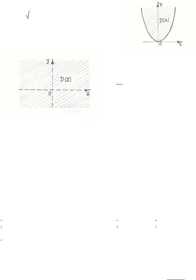
Example 1.1. Find the domain of the given function. z = f (x, y) if

b) f (x, y) =

a) f (x, y) = y − x 2

Function

Domain

D(z): y ≥ x 2

z = y − x 2

z =

D(z): xy ≠ 0

Fig. 1.1

depending on the values of the independent variables. For example, z =

	a) The domain of the function
f (x, y) =
	y − x 2 are all points of xy-plane
which are	on the parabola y = x 2 and in

the interior region of this parabola.

b) The domain of the function

z = 1 are all points of xy-plane except xy

the

points of x-axis and y-axis

2. Ways of Representation Functions of Two Variables

A function of two variables, like a function of one variable, can be specified by

atable, by a formula (analytically) or by its graph.

A.A tabular representation of a function indicates the values of the function for

anumber of pairs of values of the independent variables. For example, the table 2.1 shows dependence of area Sij on two independent variables

bi – a width and a j – a length.

	a1	a2	…	an
b1	S11	S 12	…	S 1n
b2	S 21	S 22	…	S 2n
…	…	…	…	…
bm	S m1	S m2	…	S mn

Table 2.1

B. A function of two variables can be specified by formula. In the analytical specification of a function we use a formula determining the values of the function

x2 + y2 .

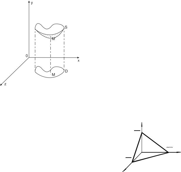
C. The function of two variables can be represented by its graph too.

The graph of a function z = f (x, y) is the collection of points (x, y, f (x, y)) and is represented by a surface S . Each point of this

surface	M ′ has		coordinates (x, y, z).	The
domain	of	the	function z = f (x, y) is the
region	D	of	xy − plane. When	point
M (x, y)	runs through region D , than			point
M ′(x, y, z)		runs through the surface S , whose
equation is z = f (x, y).

Fig.2.1

		Example				2.1.		The graph of a function
Ax + By + Cz + D = 0								is the plane passing through
					D
the points				−		, 0, 0 ,
the points				−		, 0, 0 ,
					A
		D					D
	0, −		, 0	, 0, 0, −				.
	0, −		, 0	, 0, 0, −				.
		B					A

	In Fig.2.2 is drawn the portion of this plane in	x
	the first octant.	x
	the first octant.

	D
	C
		D
	O	B
	O
D		y
A

Fig.2.2

3. A Level Curves

Let f be a function of two independent variables x and y and denote the dependent variable by z. The equation z = f (x, y) may be interpreted as defining a surface S in xyz-space. If we cut the surface with planes z = h1 , z = h2 , we get contour lines on the surface. And if we project them onto the xy-plane, we obtain a level curves f (x, y) = h1 , f (x, y) = h2 in the domain of z = f (x, y) (Fig. 3.1).

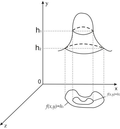
Fig. 3.1

Definition. The set of points in the xy-plane where function f (x, y) has a constant value C is called a level line of this function f (x, y) = C .

Level curves are particularly useful in engineering applications. For instance

equation z = (x − 2)2 circular plate, then distribution.

+ (y + 3)2 gave the celsius temperature at each point in a flat the level curves would be isotherms of the temperature

Example 3.1. Find the level lines of the function z = (x − 2)2 + (y + 3)2 .

Solution. The equation of the level lines of the given function is

(x − 2)2 + (y + 3)2 = C

If C takes different values, for example, C = 4, C = 9, C = 16,... we will have a family of circles with origin at a point O(2;−3) with corresponding radiuses R = 2, R = 3, R = 4,...

Example3.2. Let f (x, y) = 8 − 2x − 4 y . Sketch the graph of f, and determine the level curves.

Solution. If we let z = f (x, y), then the given equation becomes z = 8 − 2x − 4 y

This is an equation of a plane with x intercept 4, y intercept 2, and z intercept 8.

The portion of the plane in the first octant is sketched in Fig.3.2. For any value of C, the level curve

f (x, y) = C is the straight line

in the xy plane with equation 2x + 4 y − 8 + C.

The level curves are parallel lines.

Fig.3.2

4. Limits and Continuity

Definition. The limit of a function f (x, y) as (x, y) → (x0 , y0 ) is a number A if for any ε > 0 there exists a number δ > 0 such that for all points (x, y) ≠ (x0 , yo ) in

domain of f (x, y), from

x − xo

< δ

and

y − y0

< δ

follows

f (x, y) − A

< ε .

Properties of Limits

Let lim

f (x, y) = A

lim

g(x, y) = B

be given, then the

(x, y )→(x0 , y0 )

following rules hold

lim

[ f (x, y) + g(x, y)]= A + B

Sum rule

(x, y )→(x0 , y0 )

lim

[ f (x, y) − g(x, y)]= A − B

Difference rule

(x, y )→(x0 , y0 )

lim

[ f (x, y) g(x, y)]= A B

Product rule

(x, y )→(x0 , y0 )

Constant multiple rule

lim

kg(x, y) = kB , k is constant

(x, y )→(x0 , y0 )

lim

f (x, y)

if B ≠ 0

Quotient rule

(x, y )→(x0 , y0 ) g(x, y)

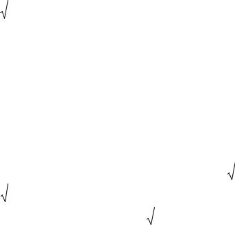
Example 4.1. Find limits of the functions:

a)lim (x2 + y2 ),

(x, y )→(3,4)

1
b) lim		,

(x, y )→(0,0) x + y

lim

x 2 + y 2

(x, y )→(0,0)

x 2

+ y 2 + 1 − 1

Solution:

lim

(x 2 + y 2 )= 32

+ (− 4)2

= 9 + 16 = 25;

(x, y )→(3,4)

lim

= ∞ ;

(x, y )→(0,0) x + y

(x2 + y2 )(

+ 1)

x2 + y2

2 + y2 + 1

lim

(

)

(

)

+ y

+ 1

( )

+ y

+ 1

− 1

x, y → 0,0

− 1 0

x, y → 0,0

lim

x2 + y2 + 1 + 1 = 2 .

(x, y )→(0,0)

Definition. A function f (x, y) is said to be continuous at the point

(x0 , y0 ) if:

f (x, y) is defined at (x0 , y0 ),

lim

f (x.y) exists,

(x, y )→(x0 , y0 )

lim

f (x, y) = f (x0 y0 ).

(x, y )→(x0 , y )

For a function

f (x, y) fair all properties of the continuous functions similar to

functions

one

variable. For example,

the

function

z =

continuous

+ y 2

everywhere,

except the

point (0,0). For

the

function

z =

the

points of

− y 2

discontinuity are all points for which y = x or y = − x .

5. Partial Increments and Derivatives of the First Order

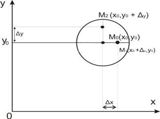
Definition. An open r-neighborhood of a given point M 0 (x0 , y0 ) is the set of all points lying inside the circle of radius r and center at the point M 0 .

Let a function z = f (x, y) be defined in a neighborhood of a point M 0 (x0 , y0 ) and

points M1 (x0 +	x, y0 ),
M 2 (x0 , y0 +	y) belong to this

neighborhood too.

Fig. 4.1

Definition.

A difference f (x0 +

x, y0 ) − f (x0 , y0 )

is called the partial

increment of the function z = f (x, y) with respect to x and is denoted by

x z .

Similarly,

f (x0 , y0 +

y) − f (x0 , y0 ) =

y z.

x z

It should be noted, that a ratio

can be considered as a function of one

x and a ratio

y z

variable with respect to

- with respect to

y .

Definition.The limit of a ratio of partial increment of the function

z = f (x, y)

with respect to

x to the increment

x ,

x tends to zero, is called a partial

derivative of function z = f (x, y) with respect to x

x z

lim

x→0

Partial derivative with respect to

of the function z = f (x, y) can be denoted

by one of the ways:

∂z

z′ ,

′ .

∂x

By analogy, lim

y z

∂z

= z

′

= f ′ .

y→0

∂y

The partial derivatives

z′

and z ′

are functions of two variables. But when we

were finding z′ we assumed that the variable

y is constant. It means that for finding

partial derivatives we can use formulas and theorems for function of the one variable.

1 / 51 2 3 4 5 > Следующая >>>

Соседние файлы в предмете [НЕСОРТИРОВАННОЕ]

#
10.02.20163.53 Mб11Ekonom_inform_konspekt_zaoch.pdf
#
12.11.201969.63 Кб0electric current_прктик_раб.doc
#
10.02.20165.42 Mб9ELMAGN_lab_2_1-4_3_1-2.doc
#
10.02.20161.1 Mб27Filosofia.docx
#
10.02.201621.48 Кб13finansovaya_strategia_predpriatia_dlya_302.docx
#
10.02.20161.51 Mб19Functions of several variables- Textbook..pdf.pdf
#
10.02.20167.06 Mб22ga2ap.doc
#
10.02.201643.9 Mб39his_uk1.pdf
#
18.08.201940.66 Кб3INDIVIDUAL_NE_ZAVDANNYa_DO_TEMI_1.docx
#
10.02.2016684.03 Кб18ISDN Основные виды обслуживания.doc
#
31.08.201925.13 Mб2ISDN Основные виды обслуживания.doc