Учебники / 0841558_16EA1_federico_milano_power_system_modelling_and_scripting

0 = iL + idc

ω˙ = (τe − τm − Dω)/2H

0 = Laf if ia − τe

where ia and if are the armature and field currents, respectively, va and vf are the armature and field voltages, respectively, ω is the rotor angular speed, τe is the electrical torque, and all other parameters are defined in Table 17.3. The coe cient D models frictions and windage losses, hence D 1 pu for τe ≈ 1 pu.

Table 17.3 Direct-current machine parameters

† Parameters required only for the compound-connected dc machine.

The typical configurations of the dc machine described above are: (i) separate winding excitation, (ii) shunt connection, (iii) series connection and (iv) compound connection. The following items provide the interface equations that make each connection type compliant with (17.2).

Separate Winding Connection

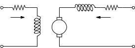
The machine is connected to two pairs of dc nodes, i.e. h-k for the armature winding and h -k for the field winding (see Figure 17.3). The voltage and current pairs (vdc, idc) and (vdc, idc) are associated with the nodes h-k and h -k , respectively. Thus, for the armature winding:

−

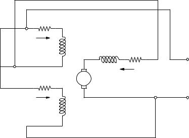
Fig. 17.4 Compound-connected dc machine equivalent circuit: (a) shunt field connected ahead the series field, and (b) shunt field connected behind the series field

Shunt-Connected DC Machine

The armature and the field windings are connected in parallel (i.e., h ≡ h and k ≡ k ). Hence:

Series-Connected DC Machine

The armature and the field windings are connected in series (i.e., k ≡ h ). Hence:

Compound-Connected DC Machine

In this case, the machine is equipped with two field windings (see Figure 17.4). The first winding is connected in series, while the second one in parallel with the armature winding. Assuming that vf and if are the voltage and the current, respectively, for the shunt-connected field winding, and vs and is are the voltage and the current, respectively, for the series-connected field winding, the DAE system becomes:

− va ωLaf ±ωLas Ra ia

ω˙ = (τe − τm − Dω)/2H

0 = Laf if ia ± Lasisia − τe

where the ± sign indicates either a cumulative or a di erential series connection. Finally, the dc-network interface constraints depend on the field circuit connections, as follows.

17.6Other Direct-Current Devices

This section describes three models of nonlinear dc devices, namely the solid oxide fuel cell, the solar photovoltaic cell and the energy battery. These devices are of growing interest for distributed and/or renewable resource generation and energy storage. Furthermore, they have interesting nonlinear DAE models, which is enough for being included in this section.

17.6.1Solid Oxide Fuel Cell

Fuel cells are a promising technology for producing electrical energy. The main issues that complicate the design of e cient and robust fuel cells are related to electrode heating and corrosion. However, fuel cells are expected to play an important role in distributed generation.

A Solid Oxide Fuel Cell (SOFC) model described in this section is based on what was proposed in [124, 159, 226, 273, 362]. Figure 17.5 depicts the

where σ = 5.670 · 10−8 W/m2/K4 is the Stefan-Boltzmann’s constant. The first equation defines the thermodynamic energy balance, while second to fifth equations defines the electrochemical reaction dynamics and the last equation defines the fuel cell voltage. In (17.22), pH2 , pO2 and pH2O are the hydrogen, oxygen and water mole fractions, respectively, qH2 , qO2 and qH2O are the hydrogen, oxygen and water flows, respectively, r is the gas constant (r = 8.314 J/mol/K), f is the Faraday constant (f = 96487 C/mol), and the remaining quantities are defined in Table 17.4. The coe cient Kr depends on the number of electrons ne in the reaction, the Faraday f constant and the current rating Idc,n = Sn/Vdc,n, as follows:

The ohmic losses modelled through the resistance Rdc are due to the resistance to the flow of ions in the electrolyte and resistance to the flow of electrons through the electrode materials. The resistance depends on the temperature Θ:

17.6.2Solar Photovoltaic Cell

Despite their high cost and low e ciency, solar photovoltaic cells are gaining in recent years popularity, thanks to the growing interest in renewable sources and, especially, thanks to public funding. At the moment, the biggest photovoltaic plant capacity is 60 MW,1 but the vast majority of solar plants have a capacity ≤ 0.2 MW. However, at least from the modelling viewpoint, photovoltaic plants are quite interesting [174, 177].

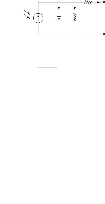
The electrical circuit is described by the following equations (see Figure 17.6):

0= vD − vdc − RSeidc

0= is(Θ)(evD /(γvΘ (Θ)) − 1) − iD

where iL is the photo-current generated by sunlight, vD and iD are the PN junction voltage and current, respectively, vΘ is the thermal potential, is is the reverse saturation current, and remaining parameters are defined in Table 17.5. The variables vΘ and is can be expressed as:

where Θ is the cell temperature and the function ϕ(Θ) is:

and kB = 1.381 · 10−23 J/K is the Boltzmann’s constant, , qε = 1.602 · 10−19 C is the electron charge, and Eg is the energy band gap, which is a function of the temperature:

The light-generated current can be linearized around a temperature of 298 K and an irradiance of 1000 W/m2:

where G is the solar irradiance or insolation in W/m2.

1This plant was completed in 2008 and is located in Olmedilla de Alarc´on, CastillaLa Mancha, Spain.

Fig. 17.6 Equivalent circuit of photovoltaic cells

Finally, the model is completed by an energy-balance di erential equation that regulates the cell heat transfer with the ambient:

+ (1 − ρc − τc − ηc)AaG − hcAc(Θ − Θa) − σεAr (Θ4 − Θa4)

where σ = 5.670 · 10−8 W/m2/K4 is the Stefan-Boltzmann’s constant and ηc is the cell power conversion e ciency:

The model described above represents a single cell. A panel is composed of a grid of cells connected in series and in parallel. Then a plant is composed of a series of several panels. However, the model above can be also used for representing the entire plant by using proper equivalent parameters. The photovoltaic cell (detailed or equivalent model) has then to be connected to the ac network. This is generally done through a VSC device and proper controllers. An example of controllers are given in Example 18.2 of Chapter 18.

In this model, the solar irradiance G is the input variable since it depends on time t, season, atmospheric conditions, dirtiness of the cell surface, etc. The solar irradiance can be provided as a series of measurements (i.e., (G, t)- value pairs) or approximated using mathematical models [33].

17.6.3Battery Energy System

Storing electrical energy is a hard task. Since capacitors are far from behaving similarly to an ideal capacitance, the only e ective way to store electrical energy is to convert it in another form of energy. For example, batteries are able to store chemical energy, pumping hydro plants store water potential energy, and flywheels store kinetic energy.2

2Example 18.3 of Chapter 18 provides another example of energy storage device based on a superconducting coil (SMES). In this case the electrical energy is converted into magnetic one.

In recent years, storage devices have gained more and more relevance because they can help systems with stochastic primary energy sources (e.g., wind or solar energy) maintain a smooth power production profile. Among the several existing energy storage devices (e.g., flywheels, electrolyzers, hydrogen storage, etc.), batteries are one of the most promising [235].

A battery is a voltage source that depends on the generated current and on the state of charge (SOC) of the battery itself. There are several battery types, e.g., lead-acid, lithium-ion, lithium-polymer, nickel-cadmium, nickelmetal hydride, zinc-air, etc. A dynamic rechargeable battery model, based on the classical Shepherd’s model, is as follows [278, 314]:

˙ −

im = (idc im)/Tm

0 = voc − vp(qe, im) + vee−βeqe − Riidc − vdc

where qe is the per unit extracted capacity normalized with respect to the maximum battery capacity Qn in Ah, im is the battery current idc passed through a low-pass filter, the polarization voltage vp(qe) depends on the sign of im, as follows: