Учебники / 0841558_16EA1_federico_milano_power_system_modelling_and_scripting

Fig. 10.1 Comparison of the transient analysis using constant impedance and constant power load models for the IEEE 14-bus system

system of the transient following the line 2-4 outage at t = 1 s. In order to dramatize the e ect of load models, the load power consumption is increased by 20% with respect to the base case. As shown in Example 16.2 of Chapter 16, the IEEE 14-bus system is unstable for such loading level and for line 2-4 outage due to the occurrence of a Hopf bifurcation. The instability drives the system trajectory to fall into a limit cycle. However, the Hopf bifurcation only occurs if using constant power load models. For constant impedance load models, the Hopf bifurcation and the consequent limit cycle disappear.

10.3.2Constant Power Factor Load

In some industrial applications, loads can be known in terms of active power consumption pL0 and power factor cos φL0. The conversion to constant PQ load is readily obtained as:

The only drawback of this kind of input data is that purely reactive loads cannot be defined. Pcos φ loads can be defined as a subclass of the PQ load class.

10.3.3Shunt Admittance

Constant shunt admittances are described by the following equations:

qh = bvh2

where g and b are the shunt conductance and susceptance, respectively. In (10.16), the susceptance b is negative for inductive charges, positive for capacitive ones. Despite the simplicity of this model, shunt admittances can be used as base class for several other devices. For example, simplified SVC models can be based on (10.16) (see Chapter 19).

In most software packages, constant admittances are included in the admittance matrix Y built for transmission lines and transformers. This practice has the advantage of reducing the computational e ort of the power flow analysis. However, there are two relevant drawbacks:

1.If shunt admittances are merged into the transmission line admittance matrix, any connection and disconnection of shunt admittances requires re-building the admittance matrix.

2.In the power flow report, shunt admittances are not considered loads but, rather, included in the transmission system losses. This may be reasonable only in case the shunt admittance is purely reactive. On the other hand, in case of modelling some active loads as constant shunt admittances, merging these loads into the admittance matrix leads to an inconsistent power flow report. In fact, active losses are computed including shunt conductance consumptions.

10.3.4Switched Shunt Admittances

A simple way to regulate the bus voltage can be obtained using a set of shunt admittances that can be switched on or o depending on the value of the voltage of the bus at which the admittances are connected. Strictly speaking, switched shunt admittances do not provide a voltage control, since admittance variations are not continuous. The base model of switched shunts is given by (10.16) but the values of g and b are not fixed and are defined using a switching logic. A possible switching rule is as follows:

b + bi, if vh − vref < Δv and b < bmax

b − bi, if vh − vref > Δv and b > 0

where vref is the assigned reference voltage, Δv is the voltage error tolerance and b is the current susceptance value and bi the susceptance value of the next element of the admittance array. The value of bi can vary if there are admittance blocks of di erent sizes. The admittance is not varied if all admittances are switched on (i.e., b = bmax) or o (e.g., b = 0). Assuming that there are s blocks and that each block has ni elements, each of which characterized by a susceptance bi, then:

i=1

The conductances gi are generally not physical resistors, but model the losses of the capacitors or reactors. In this case, the conductances gi are switched on or o if the correspondent susceptance bi is switched on or o . Finally, during time domain simulations, the switch of shunt elements are delayed by a time Δts to avoid activating too frequently admittance breakers. Table 10.10 summarizes the parameters required for defining switched shunt admittances. Other more sophisticate models of shunt devices that are able to regulate the bus voltage are described in Chapter 19.

Table 10.10 Switched shunt parameters

Chapter 11

Transmission Devices

This chapter describes the models of standard series devices, namely transmission lines (Section 11.1) and transformers (Section 11.2). In particular, Subsection 11.2.1 presents static two-winding transformers, Subsections 11.2.2 and 11.2.3 present under load tap changers and phase shifters, respectively, and Subsection 11.2.4 describes three-winding transformers. Finally, Section 11.3 discusses e cient vectorial computation for static series devices.

11.1Transmission Line

Several power system books provide a rigorous description of the determination of transmission line parameters [84, 114, 294]. In this section, it is assumed that a short line can be represented as π lumped model as shown in Figure 11.1. Short means that

where is the line length and λ is the wave length defined as:

where fn is the rated frequency of the ac system, and L and C are the perunit length inductance and capacity respectively, of the transmission line. Assuming typical values of L and C (that depend on the line geometry) and considering fn = 50 Hz, high voltage overhead transmission lines are characterized by λ ≈ 6000 km, while cables by λ (2000, 2800) km. In practice, transmission line length is never > λ/4 and the vast majority satisfies the condition < λ/8 (e.g., ≈ 750 km at 50 Hz). For ≤ λ/30, the error introduced using lumped parameters is ≤ 1%. At 50 Hz, this condition leads to ≤ 200 km. The hypothesis of short line is assumed for the remainder of this section.

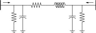
The equivalent circuit of Figure 11.1 includes a series resistance, a series reactance and four shunt elements, namely sending-end conductance and

F. Milano: Power System Modelling and Scripting, Power Systems, pp. 263–289. springerlink.com c Springer-Verlag Berlin Heidelberg 2010

Fig. 11.1 Transmission line lumped π-circuit

susceptance and receiving-end conductance and susceptance. The complex powers injected at each node are:

¯

s¯h = v¯hih (11.3)

¯ s¯k = v¯k ik

¯ ¯

According to the π model of Figure 11.1, the injected currents ih and ik can be written as:

pk = vk2(gL + gL,k) − vhvk (gL cos θhk − bL sin θhk ) qk = −vk2(bL + bL,k) + vhvk (gL sin θhk + bL cos θhk)

where θhk = θh − θk .

For short lines, gL,h ≈ gL,k ≈ 0. This assumption also derives from the di culty of evaluating shunt parasite conductances, which are generally neglected. The lumped series resistance and reactance can be computed as:

where ωs = 2πfn is the synchronous pulsation in rad/s, Zb is the base impedance in Ω and other parameters are defined in Table 11.1. The perunit length resistance R depends on the temperature, on the section and on resistivity of the conductor. The lumped shunt susceptances bL,h and bL,k can be approximated as:

Even though for standard transmission lines bL,h ≈ bL,k, it is better to maintain separated these parameters for the sake of generality. In this way, line sectioning as well as transformers can share the same programming code as transmission lines.

Table 11.1 defines all transmission line parameters. Imax, P max and Smax indicate the limits for currents, active power flows and apparent power flows. These limits are generally not required in power flow analysis, but can be used for CPF and OPF analyses (see Chapters 5 and 6 for details). Currents or apparent power limits are thermal limits. In some applications it may be required to define two or three values of such limits, depending on the emergency level and or the time that can be waited before taking a corrective action (e.g., disconnecting the line). On the other hand, active power limits generally approximate stability limits and are computed o -line base on some N-1 contingency criterion (see Subsection 5.4.5 of Chapter 5).

Table 11.1 Transmission line parameters

11.1.1Line Sections

In some cases, it may be required to define a transmission line as a series of line sections, each of which is characterized by a lumped π-circuit model as in (11.6). Sections originate from transposed lines or from connections that are composed of sections of di erent materials or characteristic parameters

(e.g., a branch composed of the series of overhead lines and underground cables). It is certainly possible to model each section as a transmission line and including fictitious buses to connect sections. However, including fictitious buses generally results in an unnecessary complication.

The equivalent model of a transmission line composed of various sections can be obtained by alternatively using the star-delta (Y - ) and the deltastar ( -Y ) transformations (see Figure 11.2). This can lead to the definition of an equivalent line whose sending and receiving-end shunt admittances are not equal.

Fig. 11.2 Equivalencing procedure for line sections: (a) original line sections; (b)-

(e) intermediate equivalents; (f) final equivalent line

For completeness, the general Y - and -Y transformation formulæ are given below (see also Figure 11.3).

1. Y - transformation:

z¯az¯b

z¯1 = z¯a + z¯b + z¯c (11.10)

z¯bz¯c

z¯2 = z¯a + z¯b + z¯c

z¯az¯c

z¯3 = z¯a + z¯b + z¯c

Fig. 11.3 Star and delta circuits used in formulæ (11.10) and (11.11)

11.1.2Tie Line

Tie lines are branches on which the active power flow is set to a given value or is bounded within assigned limits. Assuming that the active power flow is set to a constant value, the resulting model is (11.6) plus the additional equation:

Previous constraints can be easily included in an OPF problem, since generator power productions and load consumptions in case of elastic demand are not assigned. On the other hand, including (11.12) or (11.13) in the power flow problem requires that some parameter becomes a variable. At this regard, there are various possibilities.

A model consists in considering one parameter of the tie-line as a variable, for example, the series reactance xL. A very similar solution is to define a compensation variable cL, that multiplies a given series reactance, say cLxL. Considering the tie line series reactance as a variable is not an arbitrary choice. Series FACTS devices (e.g., the TCSC discussed in Chapter 19) vary the series reactance of a transmission line to impose a given active power flow.

Clearly, it is not mandatory that the new variable belongs to the tie line. For example one can use the active power of some generator (thus leading to a constant v generator model). However, in the latter case, it is more reasonable to formulate the problem as an OPF rather than as a power flow.

Example 11.1 Tie Line for the IEEE 14-Bus System

According to the base case power flow solution of the IEEE 14-bus system shown in Table 4.3 of Chapter 4, the active power flow injected at bus 4 by transmission line 2-4 is p5 = 0.5445 pu. Assume that we want to impose an active power flow injection of pref5 = 0.60 pu. Using a tie line that allows varying the series reactance can do the job. In order to obtain this result, the series reactance of line 2-4 must be x24 = 0.14624 pu. The solution of this power flow problem requires 6 iterations using a standard Newton’s method

and x(0)24 = 0.17632 as initial guess for the tie line series reactance. Imposing pref5 = 0.64 requires 9 iterations and provides x24 = 0.13402 pu, while for pref5 = 0.65, the power flow problem diverges. The critical point is the initial guess of the series reactance x24.

This simple example allows drawing a general conclusion. Series devices always create more convergence issues than shunt devices. Thus, tie line models such the one discussed in this example have to be used with caution.

11.1.3Distributed Transmission Line Models

As previously discussed, long transmission lines have to be modelled using a distributed parameter model. This leads to the well-known partial-derivative transmission line equations:

where R , L and C are defined in Table 11.1 and G is the line conductance per unit length.

Equations (11.14) and the boundary conditions:

define a boundary value problem whose general solution is too complex to be used for systems with hundreds of lines.1 Thus, some simplifications are required.

The first commonly accepted assumption is to use fast balanced timevarying phasors. The boundary value problem becomes:

1A very interesting although little exploited continuum model of power systems has been proposed in [274] and recently extended in [233].