Учебники / 0841558_16EA1_federico_milano_power_system_modelling_and_scripting

expressions of the line currents defined in (11.17) or (11.19) can be used for recomputing (11.3).2

11.1.4E ect of Frequency Variation

One of the most well accepted hypothesis of transient stability analysis is that transmission system parameters do not depend on the frequency. The assumption is that, although synchronous machine rotor speeds vary, the frequency deviations in transmission line parameters is negligible:

where Zb is the impedance base and ωs is the synchronous speed in pu (e.g., ωs = 1 pu).

Removing this assumption leads to the following equations:

ph = vh2(gL,hk(ω) + gL,h) − vhvk (gL(ω) cos θhk + bL(ω) sin θhk) (11.21) qh = −vh2(bL,hk(ω) + bL,h(ω)) − vhvk (gL(ω) sin θhk − bL(ω) cos θhk)

pk = vk2(gL(ω) + gL,k) − vhvk (gL,hk(ω) cos θhk − bL(ω) sin θhk ) qk = −vk2(bL(ω) + bL,k(ω)) + vhvk (gL(ω) sin θhk + bL(ω) cos θhk )

The value of ω can be defined in various ways. Two common choices are:

1.Computing a local frequency as the derivative of the bus phase angle. This technique is described in Section 13.4 of Chapter 13.

2.Using a system-wide frequency such as the center of inertia (COI), which is described in Subsection 15.1.9 of Chapter 15.

Example 11.2 E ect of Frequency on Line Parameters

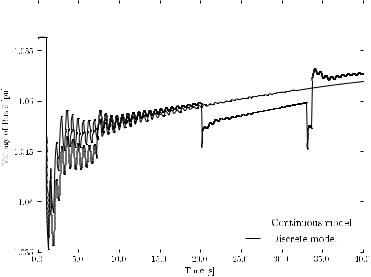
Figure 11.4 compares the numerical integration for the IEEE 14-bus system using three di erent models of transmission lines, namely (i) constant parameters as in (11.6), (ii) COI dependent parameters, and (iii) local bus frequency dependent parameters. The disturbance consists in line 2-4 outage for t = 1 s. For clarity, Figure 11.4 only shows a window from 10 to 15 s. As it can be noted, the classical approximation of using constant parameters does not introduce a significant error, at least for small variations of machine rotor speeds. Furthermore, COI and local bus approximations provides practically identical results.

2Equations (11.14) to (11.19) are in absolute values. Thus, before substituting (11.17) or (11.19) in (11.3) a proper per unit conversion has to be carried out.

Fig. 11.4 Comparison of the transient behavior of transmission lines with constant and frequency-dependent parameters for the IEEE 14-bus system.

11.1.5Coupling Device and Zero-Impedance Line

Coupling devices such as disconnecting switches or very short lines can be modelled as zero-impedance lines. Unfortunately, equations (11.6) are not adequate for modelling such coupling devices. In fact, using a very small series impedance (e.g., xL < 10−6 pu) may lead to numerical issues.

Thus, coupling devices require an ad hoc model. For example, the following model was proposed in [210]:

0 = vh − vk ph = pc

qh = qc pk = −pc qk = −qc

where the internal variables pc and qc are the active and reactive power flowing in the coupling device from bus h to bus k. The only drawback of the model (11.22) is that it does not allows putting two or more coupling devices in parallel since the powers pc and qc in each device would result indeterminate.

11.2Transformer

This section describes fixed tap and regulating twoand three-winding transformers.

11.2.1Two-Winding Transformer

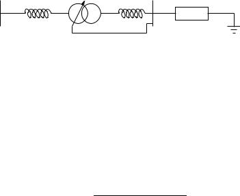
Two-winding transformers can be modelled as a transmission line with a series impedances z¯T = rT + jxT and a shunt admittance at the sending-end bus, which models iron losses gFe and the magnetizing susceptance bμ.3 Thus, substituting transformer parameters in (11.6), the following correspondences hold:

All transformer parameters are defined in Table 11.2.

Table 11.2 Transformer parameters

From the modelling viewpoint, the main di erence between transformers and transmission lines is that transformers can introduce a complex o - nominal tap ratio mejφ that allows modifying the magnitude and the phase angle of the receiving or sending-end bus voltage. For static transformers,

3Strictly speaking, a transformer should be modelled using a T model. However the error introduced by the approximated circuit is acceptable. Furthermore, in power flow analysis, transformer shunt admittances are generally neglected.

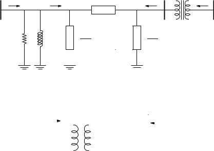
Fig. 11.7 Alternative equivalent circuit of the tap ratio module and series impedance

The same result can be obtained using the equivalent circuit shown in

¯ ¯ Figure 11.7 [2, 184]. In this case, the currents ih and ik are:

Equations (11.23) and (11.25) are obtained assuming that the tap is on the transformer primary side. Nevertheless, if the tap is on the secondary winding and the o -nominal tap ratio is m˜ = 1/m, then the admittances in (11.23) and (11.25) have to be redefined as y¯T = y¯T /m˜ 2 and y¯T = y¯T , respectively. Thus, it is important to check on which transformer side the tap changer is installed.

In conclusion, the algebraic equations of the power injections are as follows:

−vhvk (gT cos(θhk − φ) + bT sin(θhk − φ))/m qh = −vh2(bμ + bT /m2)

−vhvk (gT sin(θhk − φ) − bT cos(θhk − φ))/m

pk = vk2gT − vhvk (gT cos(θhk − φ) − bT sin(θhk − φ))/m qk = −vk2bT + vhvk (gT sin(θhk − φ) + bT cos(θhk − φ))/m

where gT + jbT = y¯T .

The fixed tap ratio unit is pu/pu since it represents the ratio of the primary voltage in pu by the secondary voltage in pu. For example, if the nominal voltages are Vn,h = 220 kV and Vn,k = 128 kV, and the actual tap positions of the transformer are Vh = 231 kV and Vk = 128 kV, the tap ratio m is:

11.2.2Under Load Tap Changer

Under Load Tap Changer (ULTC) transformers control the voltage or the reactive power varying the tap ratio. There are two models of ULTC transformers: a discrete model and a continuous one [189, 238, 241].

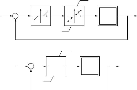
1.The discrete model consists in modelling the step ratio as a discrete variable, which can vary between the minimum and the maximum tap values mmax and mmin by a fixed step Δm. The regulator model simply switches up or down by one step Δm the tap ratio if the deviation of the regulated

quantity vk (e.g., the voltage on the secondary winding) with respect to the reference vref exceeds a given tolerance Δv, which works similarly to a dead zone (see Figure 11.8.a). The switching logic is as follows:

m + Δm, if vk − vref < Δv and m < mmax

m − Δm, if vk − vref > Δv and m > mmin

Each tap switch is a delicate process, since requires moving physically the tap position. In order to avoid unnecessary switching operations, the regulator is delayed so that a tap switch can occur only if a minimum time Δts has passed since the last switch. For this reason, ULTC controllers are relatively slow.4

2.The continuous model assumes that the tap ratio step Δm is small so that discrete switches can be approximated with a continuous variation of the tap ratio m. The time delay is approximated as a lag transfer function (see Figure 11.8.b). Hence, the tap ratio di erential equation is:

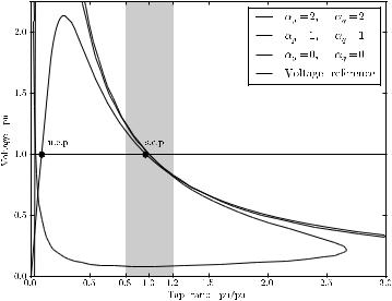
where all parameters are defined in Table 11.3 and the tap m undergoes an anti-windup limiter and the sign of the error v = vk −vref is due to the stability characteristic of the nonlinear control loop. In fact, as shown in Figure 11.10, the regulator stable equilibrium point occurs for a negative tangent slope of the ULTC-load characteristic. Example 11.3 provides a graphical proof of this statement. A similar control can be obtained by regulating the voltage of a remote bus or regulating the reactive power output of the transformer, e.g.:

4New generations of ULTC are equipped with thyristor-switched controllers, which are characterized by a fast time response.

mmax

Fig. 11.8 Voltage control diagram of the ULTC transformer: (a) discrete control and (b) continuous control

The discrete model reproduces precisely the physical behavior of the ULTC regulator. However, as discussed in Chapter 1, discrete variables complicate the analysis of DAE systems. For this reason, the continuous model is preferred for stability analysis [55]. An interesting stability study that consists in bounding the discrete behavior through an upper and a lower continuous models is proposed in [339].

Table 11.3 Under load tap changer control parameters

Example 11.4 Comparison of ULTC Discrete and Continuous

Models

Figure 11.11 shows a comparison of the transient behavior of the discrete and continuous ULTC control models. The plot is obtained substituting in the IEEE 14-bus system the fixed transformer connecting buses 4 and 9 with a voltage regulating transformer. The disturbance is line 2-4 outage at t = 1 s. For the continuous model, Kd = 0 and Ki = 0.1 1/s/pu, while for the discrete model Δv = 5%, Δm = 0.02 pu/pu and Δts = 5 s. For both models, the regulated voltage is that of bus 9, vref = 1.0563 pu, mmax = 1.2 pu/pu and mmin = 0.8 pu/pu. As expected, the behavior of the two models is similar. The discrete model introduces discontinuities in the algebraic variables (e.g., bus voltages).

11.2.3Phase Shifting Transformer

Phase Shifting Transformers (PhSTs) are able to vary the phase shifting angle φ to control the active power flow. These devices are used in meshed networks for reducing the congestion on some transmission lines and/or properly redistributing active power flows in transmission lines. A fairly complete review of PhST technologies can be found in [333]. However, regardless the PhST